Reading New York: From 3D Geometry to a Parametric City

This research investigates how existing urban geometry can inform procedural design through the extraction of footprint proportions, orientation and vertical relationships. A collection of NYC Planning Rhino models provides the source material for a computational workflow that classifies building components, normalises physical dimensions and evaluates the reliability of the resulting measurements.

The study combines a read-only census of 49 model files with a parametric massing example derived from a filtered Brooklyn dataset. RhinoCommon and Python handle extraction and geometric validation; a Grasshopper Python component translates retained area, aspect-ratio and height-proxy tuples into an adjustable urban grid. The following tutorial documents both stages for Rhino and Grasshopper users with basic Python experience.

Download the tutorial kit Read the kit instructions. The ZIP includes Python scripts, a 96-record cohort, a static Rhino snapshot, and 60 Markdown research notes. Original NYC models and bulky raw census CSVs are excluded.

1. Source data and computational environment

Get the models from the NYC Planning 3D model page and extract the archives. Keep originals in a dedicated folder. The city's metadata describes a model based on 2014 aerial imagery, organized into 59 community districts, with building envelopes distributed across unjoined footprint, roof and facade layers. This historical dataset establishes the study's temporal context.

Use Rhino 8 with its Python 3 ScriptEditor and Grasshopper. The research baseline was Rhino 8.35.26251.13001 with CPython 3.9.10. The extractor uses RhinoCommon and the Python standard library; the Grasshopper example needs no third-party plugin. MCP was used for session automation; the supplied scripts can also be executed directly in Rhino.

The source collection occupies 41.88 GB on disk. To limit memory use, the reader processes one independent File3dm at a time and disposes it before loading the next. Loaded geometry can exceed the file's disk size, so the largest individual model must still fit the available memory. A preliminary run on one small file establishes the environment before processing the full collection.

2. Geometry census and data extraction

Extract the tutorial kit somewhere writable. Open inspect_nyc.py in Rhino's Python 3 editor. Change its two configuration lines, using your own paths:

SOURCE = r"D:\NYC-models"       # extracted .3dm files directly here
OUT = r"D:\NYC-study\evidence" # fresh folder outside the models

Save the script before running it. Subfolders are not searched. The portable reader rejects an empty source folder, output inside the source folder, and an output folder already containing a census inventory. Choose a new output folder for another run. It reads the source files without adding anything to the active Rhino document.

Run the script once and keep Rhino open while the background worker runs. The editor returns after launching the worker; completion is recorded separately in the output files. Follow progress.json in the output folder. At the end, confirm status: "complete", check errors: 0, and inspect results.json for failures. Processing time depends on file size, geometry and available hardware.

Each file produces a JSON report, a footprint CSV and a height-proxy CSV. Reports include source units and tolerance, layer/type counts, exclusions, sampled geometry checks, and a full-file SHA-256. A size/modification-time comparison checks whether a file changed during the read. The hash identifies that observed copy; it cannot prove an earlier history.

From a standard Python terminal, summarize the output with the included helper:

python summarize.py "D:\NYC-study\evidence"

The source collection produces 19,320,233 object records, 648,058 eligible footprint entries, and 326,882 retained height proxies. The reader found 31 files declared in feet and 18 in millimeters. These totals provide a reference for the studied copies. Other file selections or source revisions can produce different counts under the same eligibility criteria.

3. Geometric measurements and validation

Unit normalisation. Read model.Settings.ModelUnitSystem and use RhinoMath.UnitScale to convert lengths to meters. Square that factor for areas. A factor of 304.8 between feet and millimeters becomes 92,903.04 for area; using the length factor once gives the wrong result. Keep the original coordinates and any origin transform so you can return to the source frame.

Component classification. The archive contains 8,249,164 Breps and 11,039,206 polyline curves, alongside other types. A facade patch is not a building. An open but valid roof patch is not automatically broken geometry. Layer names help identify roles, but geometry type and orientation must confirm the role.

The footprint extractor accepts closed horizontal polylines after checking degeneracy and vertical variation. Its horizontal threshold is the greater of 1 mm and ten document tolerances, converted to meters. It excludes 211,734 nonhorizontal curves, four open curves and 14 Breps in nominal footprint roles. These are eligibility decisions, not a citywide corruption count. Separate rings are not assembled into polygons with holes, and a full self-intersection audit is outside this census.

Orientation-aware footprint measurement. A rotated rectangle can occupy little of its world-axis bounding box. Aligning to its longest edge gives more useful long/short dimensions and fill ratios, though this is an approximation rather than a minimum-area rectangle. The area calculation subtracts a local origin before applying the shoelace formula, reducing cancellation from large coordinates. Across 392 comparisons with Rhino's native area calculation, the largest relative difference was approximately 8.79e-11.

Roof-to-footprint height estimation. The script associates roof surfaces with candidate footprints geometrically, using bounding-box containment and base elevation. There is no verified building identifier joining the envelopes. Roof-to-footprint vertical differences are therefore proxies. Manhattan MN05 has a median retained proxy near 50.03 m; Brooklyn BK04 is near 10.42 m. The contrast provides a basis for comparing massing characteristics, subject to incomplete matching coverage; it does not establish either district's true building-height distribution.

Read the measurement methods and district parameter reference before reusing the statistics. A pooled median footprint area of 92.27 m² is a description of eligible entries in this collection, not a universal design rule.

4. Diagnostic findings

The QN01 model demonstrates a discrepancy between layer classification and geometric orientation: a nominal footprint layer contains 209,798 nonhorizontal curves. An independent 64-object reservoir sample found facade-like upright outlines: their XY projected areas were less than 1% of their native planar areas. One concrete rectangle spans about 3.866 m vertically, has zero projected XY area, and a native planar area of about 14.359 m². Flattening every object in that layer would create misleading footprint statistics.

A separate diagnostic of the Queens parks/airports file found trim-edge deviation-to-tolerance ratios clustered near 304.8, consistent with a possible unit-conversion bookkeeping issue. The correspondence is a hypothesis about tolerance metadata rather than a confirmed account of the file's authoring history. Any repair would require object-level investigation of the physical discrepancy while preserving the source geometry.

The validity checks examined 60,627 layer-sample observations and found 49 invalid ones. The sampling scheme deliberately covers layers; it is not a uniform draw across every object. Dividing those numbers does not produce a defensible citywide defect rate. The diagnostic notes keep examples, observations and hypotheses separate.

5. Parametric urban massing in Grasshopper

The procedural stage abstracts a selected subset of the measured geometry into a new urban composition. The kit contains 96 filtered BK04 records, each retaining footprint area, aligned aspect ratio and its associated height proxy together. The selection is recorded in cohort.json: positive proxies, bounded areas and aspect ratios, and rectangle lengths small enough to fit the grid. Sorting by GUID and taking the first 96 makes the cohort reproducible; it does not make it representative.

Sampling complete tuples retains the measured association between area, aspect ratio and the matched height proxy. For area A and aspect r, the synthetic rectangle uses long = sqrt(A*r) and short = sqrt(A/r). Their product recovers A and their ratio recovers r. This simplifies the original outline, and the retained height remains a spatial inference.

1. Start a new Grasshopper definition. Use a Rhino document in meters. Add a Python 3 Script component. Use its default Script-Mode, where code runs at the top level; this example is not written for SDK/RunScript mode.
2. Name five inputs, all with Item access: n, spacing, seed, scale, height_scale. Wire every input to a number slider. Use integer sliders for n and seed.
3. Set limits and defaults. n: 1–20, default 7; spacing: 24–60, default 26 m; seed: 0–1,000,000, default 42; scale: 0.5–1.3, default 0.9; height_scale: 0.5–3, default 1.4. These are design bounds for this example, not measured zoning rules.
4. Replace the component's code with all of parametric_city.py. Its embedded cohort avoids absolute paths or external package dependencies. Name four outputs bodies, crowns, base, report.
5. Preview the result. Bodies and crowns are Brep lists; base is one Brep. Optionally connect separate Custom Preview components and colors to each geometry output. Hide the Python component's preview if you use Custom Preview. Baking is a separate, deliberate step.

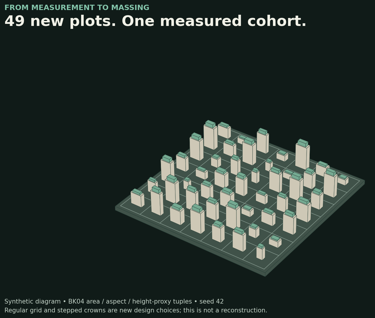
At the defaults, expect 49 bodies, 49 crowns and a 190×190×3 m square base. Each crown is 72% of its body's width and depth and adds 16% of its height. The grid and stepped crowns form the design variables introduced by the generator, while the underlying body proportions retain their relationship to the selected measurements. The code checks every output for validity and closed-solid status, and it never writes to the active Rhino document on solve.

To inspect the default geometry independently of Grasshopper, open the included Rhino snapshot in a separate document. It is a static export. The editable parametric workflow is the Python component you build above.

6. Verification and further development

Change n to 4: you should get 16 bodies, 16 crowns and a 112 m square base. Reset n to 7 and change seed to 43, then back to 42: the original numerical layout should return. Increase scale from 0.9 to 1: footprint areas grow by (1/0.9)^2, while the sampled tuples stay the same. Adjust height_scale independently to compare vertical massing while retaining footprint proportions. At the allowed limits, each rectangle remains inside its own grid cell.

RhinoCommon validation covered 4×4, 7×7 and 20×20 configurations, including maximum footprint and height scales. Reopening the default 3DM confirmed 99 valid closed solids in meters. A repeat run of the portable census reader on the small SI parks file reproduced its original hash, units, 6,486 object records and 213 eligible footprints. Aggregate results refer to the original 49-file research run; tutorial packaging included this smaller repeat check rather than a second traversal of the full 41.88 GB collection. See the verification record for remaining checks.

The current generator isolates building proportions within a regular grid. Street networks, cadastral parcels, terrain, floor counts and use remain outside its scope, and repeated cohort records do not reproduce the source district's spatial relationships. Further development will compare district cohorts, evaluate roof-matching bias and introduce explicit street and plot structures to connect individual massing characteristics with urban organisation.

The research outputs comprise reusable extraction scripts, measured parameter ranges, diagnostic examples and documented design principles. Together, these establish a reproducible reference for subsequent procedural studies. AI-assisted inspection contributes to the workflow and its documentation; it does not retrain the assistant's underlying model.

Research snapshot: 18 October 2026. Measurements and interpretations refer to the documented source collection and methods.