Conditional Volatility Forecasting:
A reusable Python module that fits rolling historical volatility, EWMA (RiskMetrics), and GARCH(1,1) to daily asset returns, forecasts conditional volatility across multiple horizons (1-, 5-, 10-, and 21-day), and benchmarks each model against realized volatility proxies using MSE, MAE, and the quasi-likelihood (QLIKE) loss. A three-state regime detector classifies each trading day as calm, normal, or stressed based on quantile thresholds applied to the fitted EWMA series. Output is exposed through a typer CLI and a Streamlit dashboard with interactive tabs for conditional vol plots, forecast-error traces, and shaded regime bands. Built on Python 3.11+ using pandas, numpy, arch, scipy, pydantic v2, plotly, and streamlit; packaged with hatchling and tested with pytest against a deterministic 500-day synthetic fixture.
I. Interactive Dashboard:
All three models — Rolling Historical, EWMA (RiskMetrics), and GARCH(1,1) — run directly in-browser on four synthetic market scenarios (generated from a seeded GARCH process). GARCH parameters are estimated via maximum-likelihood using a vectorised scipy.signal.lfilter-based filter and scipy.optimize.minimize (L-BFGS-B), and are cached after the first fit for each preset. Use the sidebar to toggle models, adjust the EWMA decay factor λ, and select a forecast horizon; the three tabs mirror the full Streamlit dashboard.
II. Project Layout:
vol-forecasting/
├── pyproject.toml                      # Build config, deps, ruff + pytest settings
├── .env.example                        # API key template
├── data/                               # Populated by scripts/download_data.py
├── scripts/
│   └── download_data.py                # Fetches prices from yfinance + FRED macro series
├── src/vol_forecasting/
│   ├── data/
│   │   ├── schemas.py                  # Pydantic v2: AssetConfig, PriceHistory
│   │   ├── fetchers.py                 # yfinance and FRED HTTP fetchers
│   │   └── loaders.py                  # CSV → validated PriceHistory schema
│   ├── models/
│   │   ├── historical.py               # Rolling std baseline + carry-forward forecast
│   │   ├── ewma.py                     # RiskMetrics EWMA (λ=0.94); flat h-step forecast
│   │   └── garch.py                    # GARCH / EGARCH / GJR-GARCH via arch package
│   ├── eval/
│   │   ├── realized.py                 # Realized vol proxies: squared return, rolling, Parkinson
│   │   ├── metrics.py                  # MSE, MAE, QLIKE, directional accuracy
│   │   └── rolling_eval.py             # Multi-horizon evaluation across all models
│   ├── regime/
│   │   └── detector.py                 # calm / normal / stressed quantile classifier
│   ├── report/
│   │   └── plots.py                    # Plotly: conditional vol, regime bands, forecast error
│   ├── cli.py                          # Typer CLI: fit | eval | regime
│   └── app.py                          # Streamlit dashboard (3 tabs)
└── tests/
    ├── conftest.py                     # Deterministic 500-day synthetic return fixture
    ├── test_models.py                  # Invariant tests: vol, EWMA, GARCH
    ├── test_eval.py                    # Realized vol proxies and metric correctness
    └── test_regime.py                  # Regime classification invariants
III. Data Layer — schemas.py & loaders.py:
PriceHistory wraps a dates-×-tickers price DataFrame and validates it at construction time via Pydantic v2. load_prices() reads a pre-downloaded CSV; fetch_prices() calls yfinance live. The .returns() method forward-fills any gaps before computing daily log changes — a necessary step for FX and crypto series with weekend holes.
# schemas.py
from __future__ import annotations
from datetime import date
from typing import Literal
import pandas as pd
from pydantic import BaseModel, field_validator, model_validator

AssetClass = Literal["equity", "etf", "fx", "crypto", "other"]

class AssetConfig(BaseModel):
    ticker: str
    asset_class: AssetClass = "equity"
    currency: str = "USD"

    @field_validator("ticker")
    @classmethod
    def normalise_ticker(cls, v: str) -> str:
        return v.strip().upper()

class PriceHistory(BaseModel):
    prices: pd.DataFrame   # dates × tickers, adjusted close
    start: date
    end: date
    model_config = {"arbitrary_types_allowed": True}

    @model_validator(mode="after")
    def validate_prices(self) -> "PriceHistory":
        if self.prices.empty:
            raise ValueError("price history is empty")
        if self.prices.isnull().all().any():
            bad = self.prices.columns[self.prices.isnull().all()].tolist()
            raise ValueError(f"all-NaN columns: {bad}")
        return self

    def returns(self, fill: bool = True) -> pd.DataFrame:
        df = self.prices.copy()
        if fill:
            df = df.ffill()
        return df.pct_change().dropna(how="all")
# loaders.py
from __future__ import annotations
from pathlib import Path
import pandas as pd
from .schemas import PriceHistory

def load_prices(path: str | Path) -> PriceHistory:
    path = Path(path)
    if not path.exists():
        raise FileNotFoundError(f"Price file not found: {path}")
    df = pd.read_csv(path, index_col=0, parse_dates=True)
    df.index = pd.to_datetime(df.index).date
    df = df.sort_index().astype(float)
    return PriceHistory(prices=df, start=df.index[0], end=df.index[-1])
IV. Model I — Rolling Historical Volatility (historical.py):
The simplest possible baseline: a rolling window standard deviation of daily returns, annualised by \(\sqrt{252}\). The \(h\)-step forecast is the current estimate carried forward unchanged — no mean-reversion, no dynamics. Despite its naivety it is a strong benchmark; it benefits from robustness to mis-specification and requires no parameter estimation. $$\hat\sigma_{t,w} = \sqrt{\frac{252}{w-1}\sum_{i=0}^{w-1}(r_{t-i} - \bar r_w)^2}$$ where \(\bar r_w\) is the window mean. The default window is \(w=21\) trading days (roughly one calendar month).
# historical.py
from __future__ import annotations
import numpy as np
import pandas as pd
from dataclasses import dataclass

_TRADING_DAYS = 252

@dataclass
class HistoricalVolResult:
    ticker: str
    vol_series: pd.Series   # rolling std, annualised
    window: int

def rolling_historical_vol(returns: pd.Series, window: int = 21,
                            annualise: bool = True) -> pd.Series:
    vol = returns.rolling(window).std(ddof=1)
    if annualise:
        vol = vol * np.sqrt(_TRADING_DAYS)
    return vol.rename("hist_vol")

def forecast_historical(vol_series: pd.Series, horizon: int = 1) -> pd.Series:
    """Carry the last rolling-std estimate forward h periods."""
    return vol_series.shift(horizon).rename(f"hist_vol_fwd{horizon}")
V. Model II — EWMA / RiskMetrics (ewma.py):
The RiskMetrics (1994) model replaces the equal-weighted window with an exponentially decaying scheme, so that recent observations receive higher weight. The variance recursion is: $$\sigma^2_t = \lambda\,\sigma^2_{t-1} + (1-\lambda)\,r_t^2$$ The decay factor \(\lambda = 0.94\) is the JP Morgan daily calibration. EWMA is structurally equivalent to IGARCH(1,1) with \(\alpha + \beta = 1\) and no intercept — meaning the process has no finite unconditional variance and the forecast is flat: \(\hat\sigma^2_{t+h|t} = \sigma^2_t\) for all \(h\). This makes EWMA fast to compute and highly responsive to large moves but unable to predict vol mean-reversion.
# ewma.py
from __future__ import annotations
import numpy as np
import pandas as pd
from dataclasses import dataclass

_TRADING_DAYS = 252

@dataclass
class EWMAResult:
    ticker: str
    vol_series: pd.Series    # annualised EWMA vol
    var_series: pd.Series    # daily variance (not annualised)
    lam: float

def fit_ewma(returns: pd.Series, lam: float = 0.94,
             annualise: bool = True) -> EWMAResult:
    """RiskMetrics EWMA: var_t = λ·var_{t-1} + (1-λ)·r_t²."""
    var = returns.ewm(alpha=1.0 - lam, adjust=False).var()
    vol = np.sqrt(var)
    if annualise:
        vol = vol * np.sqrt(_TRADING_DAYS)
    return EWMAResult(
        ticker=str(returns.name),
        vol_series=vol.rename("ewma_vol"),
        var_series=var,
        lam=lam,
    )

def forecast_ewma(result: EWMAResult, horizon: int = 1) -> pd.Series:
    """EWMA h-step forecast: flat (IGARCH persistence = 1, no mean-reversion)."""
    return result.vol_series.shift(horizon).rename(f"ewma_vol_fwd{horizon}")
VI. Model III — GARCH(1,1) (garch.py):
The Bollerslev (1986) GARCH(1,1) model adds a mean-reverting intercept to the EWMA variance recursion:
$$\sigma^2_t = \omega + \alpha\,\epsilon^2_{t-1} + \beta\,\sigma^2_{t-1}$$
The long-run (unconditional) variance is
$$\bar\sigma^2 = \frac{\omega}{1-\alpha-\beta}$$
which is finite only when \(\alpha + \beta < 1\) (stationarity). The analytical \(h\)-step forecast reverts geometrically to this long-run level:
$$\hat\sigma^2_{t+h} = \bar\sigma^2 + (\alpha+\beta)^{h-1}\!\left(\sigma^2_{t+1} - \bar\sigma^2\right)$$
This mean-reversion property is the key structural advantage of GARCH over EWMA at longer horizons: elevated volatility is expected to decay, and the speed of decay is governed by the persistence \(\alpha+\beta\). Fitting uses the arch package with MLE under Gaussian innovations; returns are scaled by 100 before fitting for numerical stability and unscaled afterward.
The module also supports EGARCH(1,1) (Nelson, 1991), which models the logarithm of variance and captures the leverage effect — negative return shocks raise volatility by more than positive shocks of equal magnitude: $$\log\sigma^2_t = \omega + \alpha\!\left(\left|\frac{\epsilon_{t-1}}{\sigma_{t-1}}\right| - \sqrt{\tfrac{2}{\pi}}\right) + \gamma\frac{\epsilon_{t-1}}{\sigma_{t-1}} + \beta\log\sigma^2_{t-1}$$ The asymmetry parameter \(\gamma < 0\) for equity series, consistent with the Black (1976) leverage hypothesis. EGARCH's log-variance specification also guarantees positivity without constraints on \(\omega, \alpha, \beta\).
# garch.py
from __future__ import annotations
import numpy as np
import pandas as pd
from dataclasses import dataclass, field
from typing import Literal

_TRADING_DAYS = 252
ModelSpec = Literal["garch", "egarch", "gjr-garch"]

@dataclass
class GARCHResult:
    ticker: str
    spec: ModelSpec
    cond_vol: pd.Series          # conditional daily vol, annualised
    long_run_var: float          # ω/(1−α−β), daily variance in decimal units
    params: dict[str, float]
    _fitted: object = field(repr=False, default=None)

def fit_garch(returns: pd.Series, spec: ModelSpec = "garch",
              p: int = 1, q: int = 1) -> GARCHResult:
    from arch import arch_model
    _SCALE = 100.0
    r = returns.dropna() * _SCALE
    if spec == "garch":
        am = arch_model(r, vol="GARCH", p=p, q=q, dist="normal")
    elif spec == "egarch":
        am = arch_model(r, vol="EGARCH", p=p, q=q, dist="normal")
    elif spec == "gjr-garch":
        am = arch_model(r, vol="GARCH", p=p, o=1, q=q, dist="normal")
    res = am.fit(disp="off", show_warning=False)
    cond_vol = pd.Series(
        res.conditional_volatility.values / _SCALE * np.sqrt(_TRADING_DAYS),
        index=returns.dropna().index, name="garch_vol",
    )
    omega = float(res.params.get("omega", np.nan)) / _SCALE**2
    alpha = float(res.params.get("alpha[1]", 0.0))
    beta  = float(res.params.get("beta[1]",  0.0))
    denom = 1.0 - alpha - beta
    long_run_var = omega / denom if denom > 1e-8 else np.nan
    return GARCHResult(
        ticker=str(returns.name), spec=spec,
        cond_vol=cond_vol, long_run_var=long_run_var,
        params=dict(res.params), _fitted=res,
    )

def forecast_garch(result: GARCHResult, horizon: int = 1) -> pd.Series:
    """σ²_{t+h} = σ̄² + (α+β)^(h−1) · (σ²_t − σ̄²). EGARCH/GJR fall back to h=1 carry."""
    if result.spec != "garch":
        return result.cond_vol.shift(horizon).rename(f"garch_vol_fwd{horizon}")
    alpha = float(result.params.get("alpha[1]", 0.0))
    beta  = float(result.params.get("beta[1]",  0.0))
    lrv   = result.long_run_var
    daily_var = (result.cond_vol / np.sqrt(_TRADING_DAYS)) ** 2
    if horizon <= 1:
        fwd = daily_var
    else:
        fwd = lrv + (alpha + beta) ** (horizon - 1) * (daily_var - lrv)
    return (np.sqrt(fwd.clip(lower=0)) * np.sqrt(_TRADING_DAYS)
            ).shift(horizon).rename(f"garch_vol_fwd{horizon}")
VII. Realized Volatility Proxies (realized.py):
Forecasting accuracy requires a realized volatility target. Daily conditional variance models cannot be evaluated against a single squared return (too noisy), so three proxies are provided:
| Proxy | Formula | Notes |
|---|---|---|
| Squared return | \(rv_t = 252 \cdot r_t^2\) | Unbiased but high variance. Standard in academic work. |
| Rolling RV | \(rv_{t,w} = \sqrt{\frac{252}{w}\sum_{i=0}^{w-1}r_{t-i}^2}\) | Smoothed proxy; reduces noise but introduces look-back bias. |
| Parkinson (1980) | \(rv_t^P = \sqrt{\frac{252}{4\ln 2}(\ln H_t/L_t)^2}\) | Up to 5× more efficient than close-to-close when OHLC data is available. |
| Forward \(h\)-day RV | \(rv_{t,h} = \sqrt{\frac{252}{h}\sum_{i=1}^{h}r_{t+i}^2}\) | The primary evaluation target: aligns with an \(h\)-step-ahead forecast made at \(t\). |
# realized.py
from __future__ import annotations
import numpy as np
import pandas as pd

_TRADING_DAYS = 252

def rolling_realized_vol(returns: pd.Series, window: int = 21) -> pd.Series:
    rv = returns.rolling(window).apply(
        lambda x: np.sqrt(np.mean(x**2) * _TRADING_DAYS), raw=True
    )
    return rv.rename("rv_roll")

def parkinson_vol(high: pd.Series, low: pd.Series, window: int = 21) -> pd.Series:
    hl2 = (np.log(high / low) ** 2) / (4.0 * np.log(2.0))
    return np.sqrt(hl2.rolling(window).mean() * _TRADING_DAYS).rename("rv_parkinson")

def horizon_realized_vol(returns: pd.Series, horizon: int = 1) -> pd.Series:
    """Forward-looking h-day realized vol: rv[t] covers returns t+1 through t+h."""
    sq = returns ** 2
    fwd_sum = sq[::-1].rolling(horizon).sum()[::-1]
    return np.sqrt(fwd_sum * _TRADING_DAYS / horizon).shift(-horizon).rename(f"rv_fwd{horizon}")
VIII. Evaluation Framework (metrics.py & rolling_eval.py):
Three loss functions are computed for each model-horizon pair:
| Loss | Formula | Properties |
|---|---|---|
| MSE | \(\mathbb{E}[(\hat\sigma_h - rv_h)^2]\) | Penalises large errors quadratically; sensitive to outliers. |
| MAE | \(\mathbb{E}[|\hat\sigma_h - rv_h|]\) | Robust to extreme realized-vol spikes. |
| QLIKE | \(\mathbb{E}\!\left[\log\hat\sigma^2 + rv/\hat\sigma^2\right]\) | Scale-invariant; the standard loss in Patton (2011) for robust volatility ranking. Lower is better. |
Directional accuracy measures the fraction of periods where the model correctly predicts whether volatility will rise or fall. rolling_eval() fits each model once on the full return history (GARCH conditional variance is a filtered, one-sided estimate at each point) and then aligns the \(h\)-step forecast series against the corresponding forward-realized vol proxy.
# metrics.py
from __future__ import annotations
from dataclasses import dataclass
import numpy as np
import pandas as pd

@dataclass
class EvalMetrics:
    model: str; horizon: int
    mse: float; mae: float; qlike: float
    directional_accuracy: float; n_obs: int

def mse(forecast: np.ndarray, realized: np.ndarray) -> float:
    m = np.isfinite(forecast) & np.isfinite(realized)
    return float(np.mean((forecast[m] - realized[m]) ** 2))

def qlike(forecast: np.ndarray, realized: np.ndarray) -> float:
    """QLIKE = E[log σ² + rv/σ²]. Scale-invariant; robust for vol model ranking."""
    m = np.isfinite(forecast) & np.isfinite(realized) & (forecast > 0) & (realized > 0)
    return float(np.mean(np.log(forecast[m]) + realized[m] / forecast[m]))

def directional_accuracy(forecast: np.ndarray, realized: np.ndarray,
                          prev: np.ndarray) -> float:
    m = np.isfinite(forecast) & np.isfinite(realized) & np.isfinite(prev)
    return float(np.mean(np.sign(forecast[m] - prev[m]) == np.sign(realized[m] - prev[m])))
# rolling_eval.py (key section)
def rolling_eval(returns: pd.Series,
                 horizons: tuple[int, ...] = (1, 5, 10, 21),
                 window: int = 21,
                 fit_garch_flag: bool = True) -> list[RollingEvalResult]:
    ewma_res  = fit_ewma(returns)
    garch_res = fit_garch(returns) if fit_garch_flag else None

    results = []
    for h in horizons:
        rv   = horizon_realized_vol(returns, horizon=h)
        hist = rolling_historical_vol(returns, window=window)
        models = {
            "historical": forecast_historical(hist,      horizon=h),
            "ewma":       forecast_ewma(ewma_res,        horizon=h),
        }
        if garch_res is not None:
            models["garch"] = forecast_garch(garch_res, horizon=h)

        forecasts_df = pd.DataFrame(models).dropna(how="all")
        rv_aligned   = rv.reindex(forecasts_df.index)
        metrics = [evaluate(name, forecasts_df[name], rv_aligned, h)
                   for name in forecasts_df.columns]
        results.append(RollingEvalResult(
            ticker=str(returns.name), horizon=h,
            metrics=metrics, forecasts=forecasts_df, realized=rv_aligned,
        ))
    return results
IX. Volatility Regime Detector (detector.py):
The regime classifier applies full-sample quantile thresholds to the EWMA conditional vol series:
$$\text{regime}_t = \begin{cases}\textit{calm} & \sigma_t \le Q_{0.25} \\ \textit{stressed} & \sigma_t \ge Q_{0.75} \\ \textit{normal} & \text{otherwise}\end{cases}$$
The 25th and 75th percentiles are computed on the full fitted series; the resulting labels are used for regime-band overlays on the time-series plots. By default the three buckets each cover roughly 25%, 50%, and 25% of observations — a deliberate choice that maps to the tails of the empirical vol distribution rather than to calendar-defined episodes. The thresholds can be overridden with custom quantiles at the call site. regime_summary() reports days and percentage of sample in each state.
# detector.py
from __future__ import annotations
import pandas as pd
from dataclasses import dataclass
from typing import Literal

RegimeLabel = Literal["calm", "normal", "stressed"]

@dataclass
class RegimeResult:
    ticker: str
    labels: pd.Series              # calm / normal / stressed per date
    vol_series: pd.Series
    thresholds: dict[str, float]   # calm_cap, stressed_floor (annualised vol)

def detect_regimes(vol_series: pd.Series,
                   calm_q: float = 0.25,
                   stressed_q: float = 0.75) -> RegimeResult:
    vol = vol_series.dropna()
    calm_cap       = float(vol.quantile(calm_q))
    stressed_floor = float(vol.quantile(stressed_q))
    labels = pd.Series("normal", index=vol.index, name="regime", dtype=object)
    labels[vol <= calm_cap]       = "calm"
    labels[vol >= stressed_floor] = "stressed"
    return RegimeResult(
        ticker=str(vol_series.name), labels=labels, vol_series=vol,
        thresholds={"calm_cap": calm_cap, "stressed_floor": stressed_floor},
    )

def regime_summary(result: RegimeResult) -> pd.DataFrame:
    counts = result.labels.value_counts().rename("days")
    pct    = (counts / counts.sum() * 100).round(2).rename("pct")
    return pd.DataFrame({"days": counts, "pct": pct}).reindex(
        ["calm", "normal", "stressed"]
    ).fillna(0)
X. Visualization (plots.py):
Three Plotly figures are produced by the report module and embedded in the Streamlit dashboard. Conditional vol: all model series overlaid with a dotted realized-vol reference line. Regime bands: shaded background rectangles (green/yellow/red) over the EWMA series, drawn by iterating through contiguous runs of the same label. Forecast error: absolute error per model, smoothed with a 21-day moving average, on a shared axis for direct comparison.
# plots.py (regime-band section)
def plot_regime_bands(vol_series: pd.Series, labels: pd.Series,
                      title: str = "Volatility Regimes") -> go.Figure:
    _FILL = {"calm":     "rgba(52, 168, 83,  0.14)",
             "normal":   "rgba(251, 188, 5,  0.10)",
             "stressed": "rgba(234, 67,  53, 0.18)"}
    fig = go.Figure()
    fig.add_trace(go.Scatter(x=vol_series.index, y=vol_series.values,
                             name="EWMA Vol", line=dict(color="#EF553B", width=1.5)))
    current, band_start = labels.iloc[0], vol_series.index[0]
    for dt, regime in labels.items():
        if regime != current:
            fig.add_vrect(x0=band_start, x1=dt, fillcolor=_FILL[current],
                          layer="below", line_width=0)
            band_start, current = dt, regime
    fig.add_vrect(x0=band_start, x1=vol_series.index[-1],
                  fillcolor=_FILL[current], layer="below", line_width=0)
    fig.update_layout(title=title, xaxis_title="Date",
                      yaxis_title="Annualised Vol", template="plotly_white")
    return fig
XI. CLI — cli.py:
Three subcommands share a common --prices-file / --ticker / --window interface. When --prices-file is omitted the engine fetches live data from yfinance.
# cli.py (key subcommands)
@app.command("fit")
def cmd_fit(ticker: str = "SPY", model: str = "garch",
            prices_file: Optional[Path] = None, window: int = 252) -> None:
    """Fit a volatility model and print a conditional vol summary."""
    returns = _load_returns(ticker, prices_file, window)
    res = fit_garch(returns, spec=model)   # or fit_ewma / rolling_historical_vol
    console.print(f"Persistence (α+β): {res.params['alpha[1]'] + res.params['beta[1]']:.4f}")
    console.print(f"Long-run vol:       {(res.long_run_var * 252) ** 0.5:.2%}")
    # ... rich table with latest / mean / min / max vol

@app.command("eval")
def cmd_eval(ticker: str = "SPY", horizons: str = "1,5,10,21", ...) -> None:
    """Walk-forward evaluation across models and forecast horizons."""
    # prints a rich.Table per horizon: model | MSE | MAE | QLIKE | Dir.Acc. | N

@app.command("regime")
def cmd_regime(ticker: str = "SPY", ...) -> None:
    """Classify volatility into calm / normal / stressed regimes."""
    # prints regime counts + thresholds; colour-coded green/yellow/red
Usage:
# Install
pip install -e ".[dev]"

# Fit GARCH(1,1) to SPY (live fetch from yfinance)
vol-forecast fit --ticker SPY --model garch

# Evaluate all three models across 1-, 5-, 10-, and 21-day horizons (offline)
vol-forecast eval --ticker SPY --prices-file data/prices_yfinance.csv --horizons 1,5,10,21

# Regime map for BTC-USD
vol-forecast regime --ticker BTC-USD --prices-file data/prices_yfinance.csv

# Launch Streamlit dashboard
streamlit run src/vol_forecasting/app.py
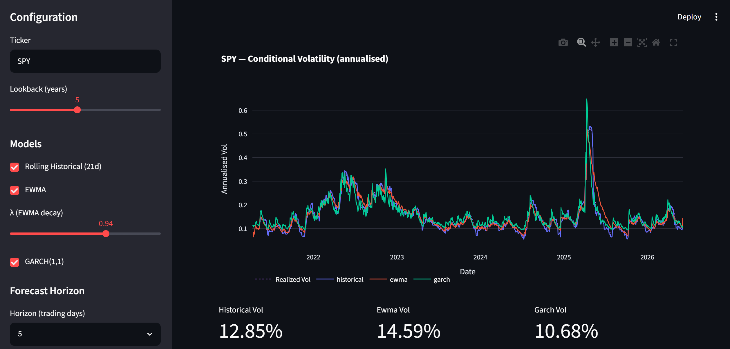
XII. Streamlit Dashboard (app.py):
The dashboard exposes the full module via a browser UI. The sidebar controls ticker, lookback period, model selection, \(\lambda\), and forecast horizon. Three tabs present the output: Conditional Volatility overlays all fitted series and the rolling realized-vol reference, with metric cards showing the latest annualised level per model; Forecast Error plots the 21-day moving-average absolute error per model and renders the evaluation metrics table; Regime Map draws the shaded regime-band chart and shows a three-column breakdown of days and percentages per state.
Setup and launch:
# 1. Navigate to the project root
cd assets/projects/vol_forecasting

# 2. Create and activate a virtual environment (Python 3.11+ required)
python -m venv .venv
# Windows:
.venv\Scripts\Activate.ps1
# macOS / Linux:
source .venv/bin/activate

# 3. Install the package and all dependencies
pip install -e ".[dev]"

# 4. (Optional) copy the env template and add a FRED API key
cp .env.example .env

# 5. Launch
streamlit run src/vol_forecasting/app.py
Streamlit starts a local server at http://localhost:8501 and opens it in the default browser. Data is fetched live from Yahoo Finance on first load and cached for one hour; changing the ticker or lookback invalidates the cache and triggers a fresh fetch. GARCH(1,1) fitting takes 2–5 seconds per series and is re-run whenever the ticker or lookback changes. To work fully offline, first run python scripts/download_data.py (which writes data/prices_yfinance.csv), then swap the load_data call in app.py to use load_prices("data/prices_yfinance.csv") from vol_forecasting.data.loaders.
Sidebar controls:
| Control | Default | Effect |
|---|---|---|
| Ticker | SPY | Any yfinance-valid symbol: QQQ, BTC-USD, EURUSD=X, ^VIX, etc. |
| Lookback (years) | 5 | 1–10 years of daily price history fetched from yfinance |
| Rolling Historical | on | Toggles the 21-day rolling std baseline |
| EWMA | on | Toggles the RiskMetrics exponentially weighted estimator |
| λ (EWMA decay) | 0.94 | Lower values react faster to new shocks; 0.94 is the JP Morgan daily calibration |
| GARCH(1,1) | on | Fits the full GARCH model via MLE (2–5 s); uncheck to skip |
| Horizon (trading days) | 5 | Sets the forecast horizon for the Forecast Error tab: 1, 5, 10, or 21 days |
| Tab | Content |
|---|---|
| 📈 Conditional Volatility | All fitted vol series overlaid with a dotted rolling-realized-vol reference line. Metric cards below show the latest annualised conditional vol for each active model. |
| 📉 Forecast Error | Absolute error \(|\hat\sigma_{t+h} - rv_{t+h}|\) per model, smoothed with a 21-day moving average. Below the chart: a summary table of MSE, MAE, QLIKE, directional accuracy, and observation count for each model at the selected horizon. |
| 🗺️ Regime Map | EWMA vol series with shaded regime bands (green = calm, yellow = normal, red = stressed). Below: three metric tiles with days and % of sample per regime, and the quantile thresholds used for classification. |
# app.py (structure)
st.set_page_config(page_title="Volatility Forecasting", layout="wide")

with st.sidebar:
    ticker   = st.text_input("Ticker", "SPY")
    lookback = st.slider("Lookback (years)", 1, 10, 5)
    use_hist  = st.checkbox("Rolling Historical (21d)", value=True)
    use_ewma  = st.checkbox("EWMA", value=True)
    lam       = st.slider("λ (EWMA decay)", 0.85, 0.99, 0.94)
    use_garch = st.checkbox("GARCH(1,1)", value=True)
    horizon   = st.selectbox("Horizon (trading days)", [1, 5, 10, 21], index=1)

tab1, tab2, tab3 = st.tabs(
    ["📈 Conditional Volatility", "📉 Forecast Error", "🗺️ Regime Map"]
)
# tab1: plot_conditional_vol() + per-model metric cards
# tab2: rolling_eval() → plot_forecast_error() + evaluation metrics table
# tab3: detect_regimes() → plot_regime_bands() + 3-column regime breakdown
XIII. Test Suite:
All tests are fully offline. The shared sample_returns fixture in conftest.py generates a deterministic 500-day SPY-like return series using numpy.random.default_rng(42). Tests verify mathematical invariants (vol non-negativity, annualisation factor, GARCH persistence < 1, long-run variance positivity, regime percentages summing to 100%) and structural properties (forecast shifts align, h=21 GARCH forecast closer to long-run vol than h=1).
# conftest.py
@pytest.fixture
def sample_returns() -> pd.Series:
    """Deterministic 500-day log-normal SPY-like return series (seed 42)."""
    rng = np.random.default_rng(42)
    dates = pd.bdate_range("2022-01-01", periods=500)
    return pd.Series(rng.normal(0.0004, 0.011, size=500), index=dates, name="SPY")
# test_models.py — selected invariants
class TestEWMA:
    def test_higher_lambda_smoother(self, sample_returns):
        """Higher λ → slower adaptation → lower std of daily vol changes."""
        res_low  = fit_ewma(sample_returns, lam=0.90)
        res_high = fit_ewma(sample_returns, lam=0.99)
        assert res_high.vol_series.diff().std() < res_low.vol_series.diff().std()

class TestGARCH:
    def test_persistence_less_than_one(self, sample_returns):
        res = fit_garch(sample_returns)
        assert res.params["alpha[1]"] + res.params["beta[1]"] < 1.0

    def test_forecast_reverts_to_long_run(self, sample_returns):
        """h=21 forecast should be closer to long-run vol than h=1 forecast."""
        res   = fit_garch(sample_returns)
        fwd1  = forecast_garch(res, horizon=1).dropna()
        fwd21 = forecast_garch(res, horizon=21).dropna()
        lr_vol = math.sqrt(res.long_run_var * 252)
        idx = fwd1.index.intersection(fwd21.index)
        assert (fwd21[idx] - lr_vol).abs().mean() < (fwd1[idx] - lr_vol).abs().mean()

# test_regime.py
class TestRegimeDetector:
    def test_summary_percentages_sum_to_100(self, sample_returns):
        res    = fit_ewma(sample_returns)
        regime = detect_regimes(res.vol_series.dropna())
        assert abs(regime_summary(regime)["pct"].sum() - 100.0) < 0.1
XIV. Configuration & Data Sources:
| Variable | Default | Description |
|---|---|---|
DATA_SOURCE | yfinance | Live-fetch source when --prices-file is omitted |
FRED_API_KEY | (none) | Required for FRED macro overlay download (FRED is optional) |
File generated by download_data.py | Source | Coverage |
|---|---|---|
prices_yfinance.csv | Yahoo Finance | 5 years, 9 tickers: SPY, QQQ, IWM, GLD, TLT, USO, BTC-USD, EURUSD=X, ^VIX |
fred_macro.csv | FRED | 5 years, 5 series: Fed Funds, 10Y−2Y, HY OAS, VIX (FRED), CPI |
Team:
Theodosios Dimitrasopoulos, personal project.
Tools & methods:
Python 3.11, pandas, NumPy, SciPy, arch (GARCH/EGARCH/GJR-GARCH via MLE), Pydantic v2 (schema validation), Typer (CLI), rich (console output), Plotly (interactive figures), Streamlit (dashboard), yfinance / FRED (market data), pytest, ruff, hatchling. Volatility methodology: rolling window std (baseline), RiskMetrics EWMA (\(\lambda=0.94\), IGARCH(1,1)), GARCH(1,1) and EGARCH(1,1) with Gaussian innovations; multi-horizon analytical mean-reversion forecasts; MSE, MAE, and QLIKE loss evaluation against forward-looking realized vol proxies; quantile-based three-state regime detector.