Long/Short Global Macro Strategies with Target Beta Using the Three-Factor Model:
ABSTRACT— This project involves the construction of a Long/Short Global Macro strategy based on Fama-French Three-Factor Model with a target beta and the evaluation of its sensitivity to variation of Beta and the length of the estimation terms for the covariance matrix and the expected returns under different market scenarios. Several comparisons are drawn between different target betas as well as different term structures.
KEYWORDS— Global Macroeconomic Trends, Long/Short, French, Fama, Beta, Three-Factor Model, Trading Strategies, Portfolio Management
GOOGLE COLAB OVERVIEW— This is the complete design and implementation docs in a Google Colab notebook,
I. INTRODUCTION
A. Fama-French Three-Factor Model
Historically, Fama-French Three-Factor Model is regarded as a development of CAPM which explains a relationship between expected returns and risk factors. Sharpe, Lintner, and Black developed an asset pricing model referred as CAPM which illustrates expected returns on the securities are a positive linear function of market beta. The CAPM, developed theoretically, had an empirical success, and became the standard model for describing the cross-sectional structure of expected returns on equity. However, some researchers revealed there were some anomalies that cannot be explained by the CAPM. Banz found the market equity had a relationship between expected returns. Stocks with smaller market equity had higher rates of return, usually referred to as the small cap effect. Bhandari found leverage helps explain the cross-section of average stock returns. Stattman, Rosenberg, Reid and Lanstein found that average returns on U.S stocks were positively related to the ratio of a firm’s book value of common equity to its market value.
In response to this criticism, Eugene Farmer, and Kenneth French, in a paper published in 1992, empirically showed that the four representative anomaly factors discovered at the time in the U.S. stock market: market equity, book-to-market ratio, leverage, and E/P (the inverse of P/E ratio), were aggregated into market equity and book-to-market ratio.
They advanced their study and proposed Fama-French Three-Factor model which describes a cross section of average stock returns with three factors, market risk premium, market equity, and book-to-market ratio.
Under the Fama-French Three-Factor model, the random return of security is given by the following formula,
\begin{equation} \boxed{r_{i}-r_{f}=\alpha_{i}+\beta_{i}^{MKT}(r_{m}-r_{f})+\beta_{i}^{SMB}r_{i}^{SMB}+\beta_{i}^{HML}r_{i}^{HML}+\epsilon_{i}} \end{equation}
\begin{equation} \boxed{R_{i}-r_{f}=\alpha_{i}+\beta_{i}^{MKT}(R_{M}-r_{f})+\beta_{i}^{SMB}R_{SMB}+\beta_{i}^{HML}R_{HML}} \end{equation}
B. Markowitz Portfolio
Markowitz portfolio theory also known as modern portfolio theory is a theory on how risk-averse investors can construct portfolio to maximize expected return based on a given level of market risk. The theory can also be used to construct a portfolio that minimize risk for a given level of expected return,
\begin{cases} \min\limits_{\omega}\omega^{T}\Sigma\omega \\ e^{T}\omega=1 \\ \rho^{T}\omega=\rho_{T} \\ \end{cases}
where \(\omega\) is the vector of weights of the portfolio securities, \(\Sigma\) is the covariance matrix , \(\rho\) is the expected return, \(\rho_{T}\) is the target return.
C. Linear Regression
An approach for predicting a quantitative response \(Y\) and the basis of multiple predictor variable \(X_{j}\) that assume an approximately linear relationship between \(X_{j}\) and \(Y\). For a model with \(p\) predictors, the linear regression takes the form,
\begin{equation} Y=\beta_{0}\sum_{j=1}^{p} \beta_{j}X_{j}+\epsilon \end{equation}
\begin{equation} \hat{f}(X)=\hat{\beta_{0}}+\sum_{j=1}^{p} \hat{\beta_{j}}X_{j} \end{equation}
\begin{equation} RSS=\sum_{i=1}^{n} (y_{i}-\hat{\beta_{0}}-\sum_{j=1}^{p} \hat{\beta_{j}}X_{j})^{2} \end{equation}
II. INVESTMENT UNIVERSE AND BACKTESTING
A. Data
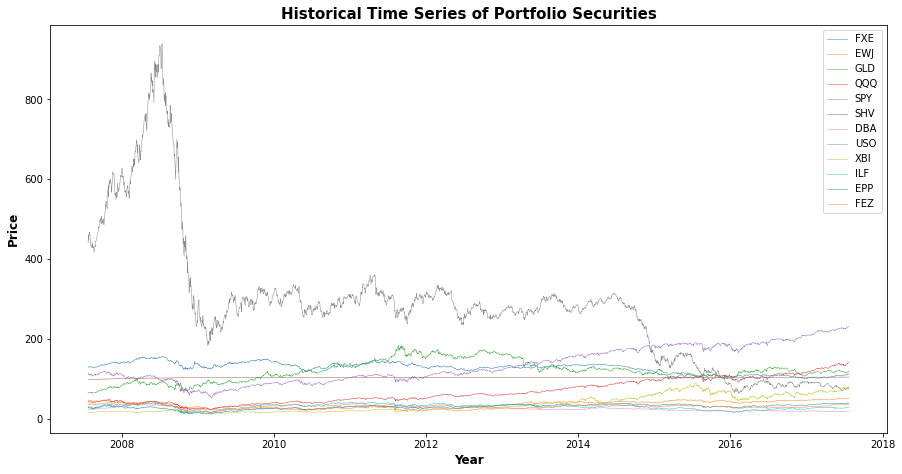
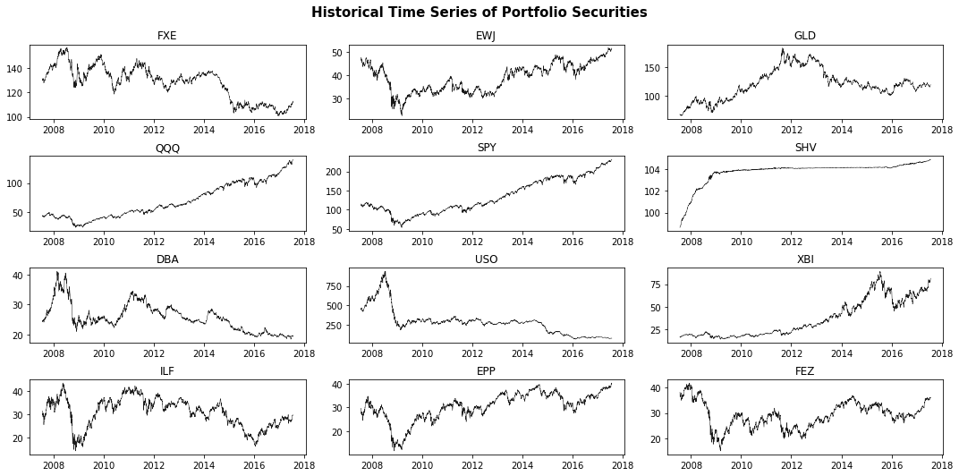
We used the 12 ETFs belowfrom March 1, 2007 to June 30, 2020:
- CurrencyShares Euro Trust (FXE)
- iShares MSCI Japan Index (EWJ)
- SPDR GOLD Trust (GLD)
- PowerShares NASDAQ-100 Trust (QQQ)
- SPDR S&P500 (SPY)
- iShares Lehman Short Treasury Bond (SHV)
- PowerShares DB Agriculture Fund (DBA)
- United States Oil Fund LP (USO)
- SPDR S&P Biontech (XBI)
- iShares S&P Latin America 40 Index (ILF)
- iShares MSCI Pacific ex-Japan Index Fund (EPP)
- SPDR DJ Euro Stoxx 50 (FEZ)
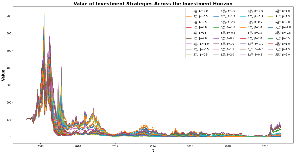
B. Investment Horizon
The investment horizon was divided into the following sub-periods,
- Pre-Subprime Crisis : March 22, 2007 – March 3, 2008
- During Subprime Crisis : March 3, 2008 – September 10, 2010
- Post-Subprime Crisis : September 10, 2010 – January1, 2015
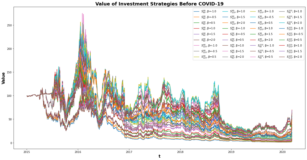
- Pre-COVID-19 Pandemic : January 1, 2015 – March 9, 2020
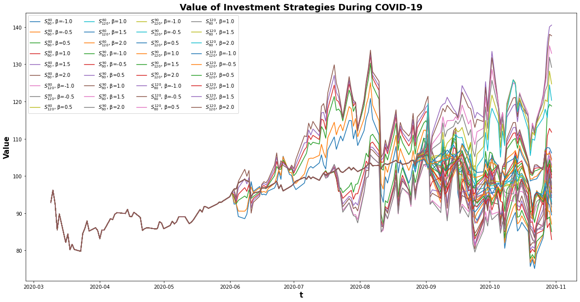
- During COVID-19 Pandemic : March 9, 2020 – October 30, 2020
Individual backtests were executed for each sub-period to compare strategies. We compared with different perspectives.
- Impact on Beta Target: Compared our strategy in terms of target beta in the same sub-period. Changed target beta \(\beta_{T}^{m}\), and compare performance.
- Impact of various term structure given Beta: Compare portfolios’ performance with different term structures and fixed beta. \(S_j^{i}\) represents a term structure with \(i\) days lookback period to estimate the expected return and \(j\) days lookback period to estimate the covariance matrix.
III. INVESTMENT STRATEGY
A. Objective Function
We consider the following investment strategy,
\begin{cases} \max\limits_{\omega} \rho^{T}\omega-\lambda(\omega-\omega_{p})^{T}\Sigma(\omega-\omega_{p}) \\ \sum_{i=1}^{n} \beta_{i}^{m}\omega_{i}=\beta_{T}^{m} \\ \sum_{i=1}^{n} \omega_{i}=1 \end{cases}
- \(\omega_{i}\): weight allocated to each security \(S_{i}\),
- \(\omega\) is a vector of weights,
- \(\rho\): vector of expected returns of security \(S_{i},
- \(\Sigma\): The covariance matrix between securities reuturns derived from the factor model,
- \(\omega_{p}\): composition of a reference Portfolio, the previous portfolio when rebalancing the portfolio,
- \(\beta_{i}^{m}=\frac{cov(r_{i},r_{M})}{\sigma^{2}(r_{M})}\): the Beta of security \(S_{i}\) as defined in the CAPM model,
- \(\beta_{T}^{m}\): the portfolio's target beta.
B. Term Structures
We investigated the following term structures,
\begin{equation} \begin{cases} S_{60}^{60} \\ S_{120}^{60} \\ S_{60}^{90} \\ S_{120}^{90} \\ S_{60}^{120} \\ S_{120}^{120} \end{cases} \end{equation}
C. Target Beta
We investigated combinations of the term structures and the following target \(\beta\)'s,
\begin{equation} \beta_{T}^{m}=\begin{cases} -1.0 \\ -0.5 \\ 0.5 \\ 1.0 \\ 1.5 \\ 2.0 \end{cases} \end{equation} D. Performance Metrics
The trading strategy pipeline performs computations of the following performance metrics,
- Cumulated Return
- Annual Arithmetic Mean / Geometric Mean Return
- Annual Min Return
- Max 10-days Drawdown
- Sharpe Ratio
E. Risk Metrics
The trading strategy pipeline also performs computations of the following risk metrics,
- Volatility
- Daily VaR
- Annual VaR
- Modified VaR
- Annual CVaR
- Skewness
- Kurtosis
IV. RESULTS & DISCUSSION
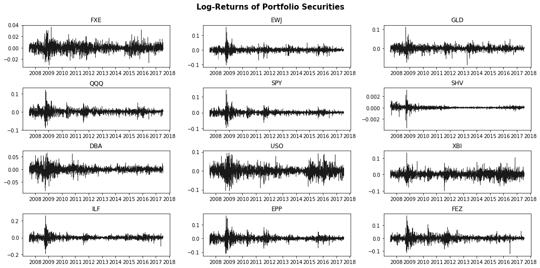
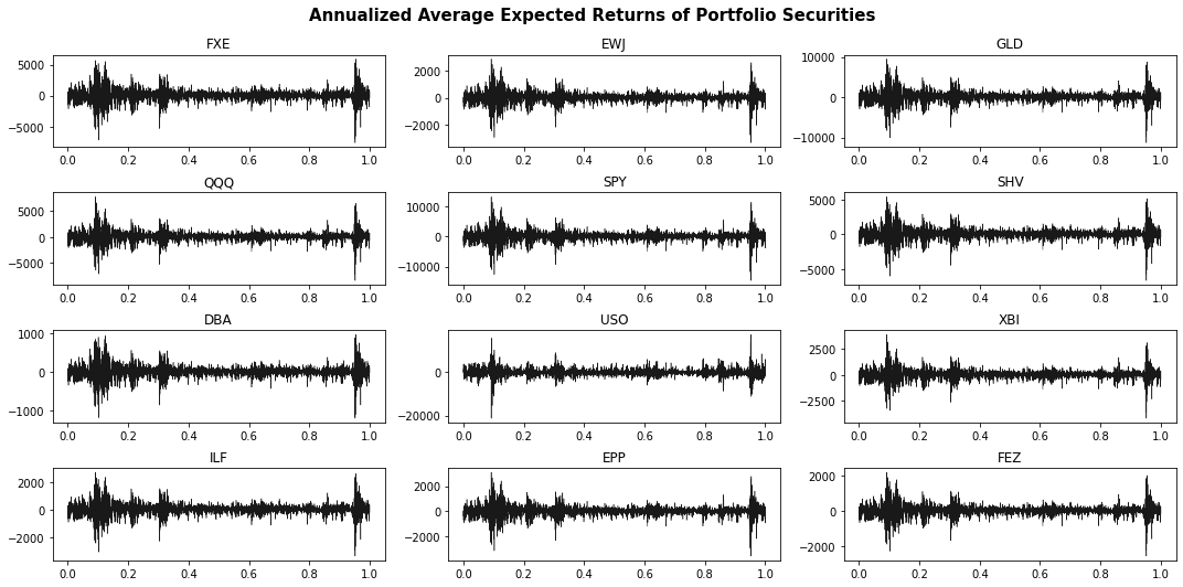
A. Return on Investment
The returns and log-returns of the portfolio securities are summarized below,
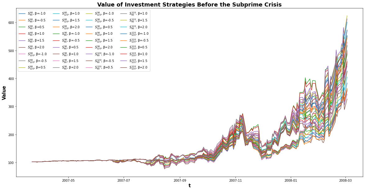
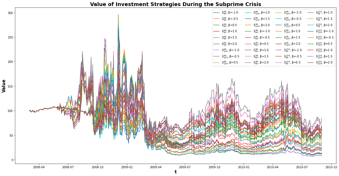
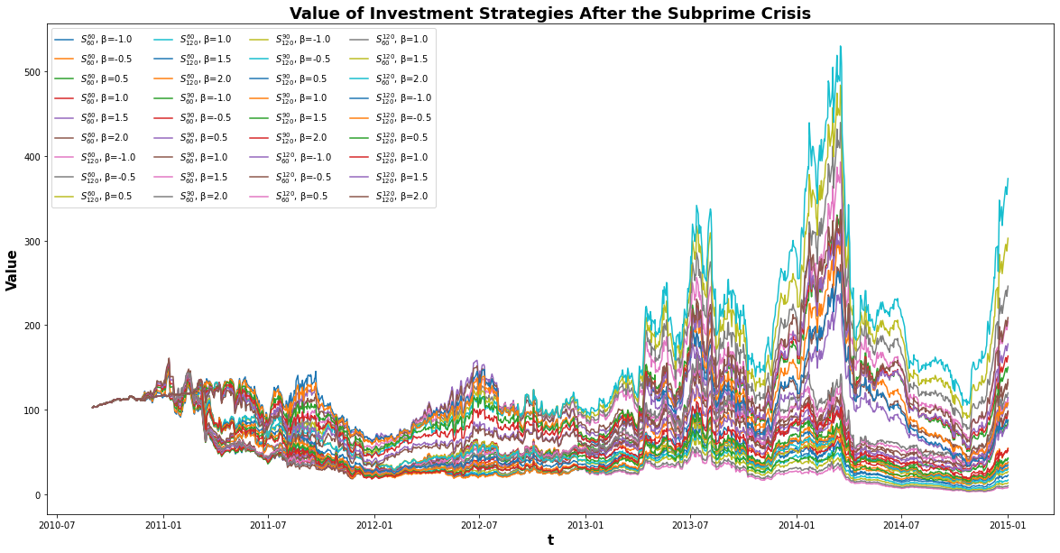
B. PnL
The evolution of cumulated daily Profit and Loss as summing with an initial investment of $100 on the first allocation date is as follows,
C. Distribution of Daily Returns
The following plots show the distribution of daily returns for different term structures and \(\beta\)'s (Click on the right/left side of each slideshow to go to the next/previous plot),
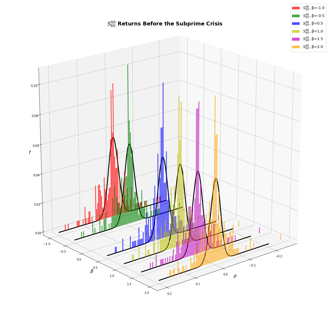
Fig. 12: The distribution of returns from the \(S_{60}^{60}\) investment strategy before the Subprime Crisis.
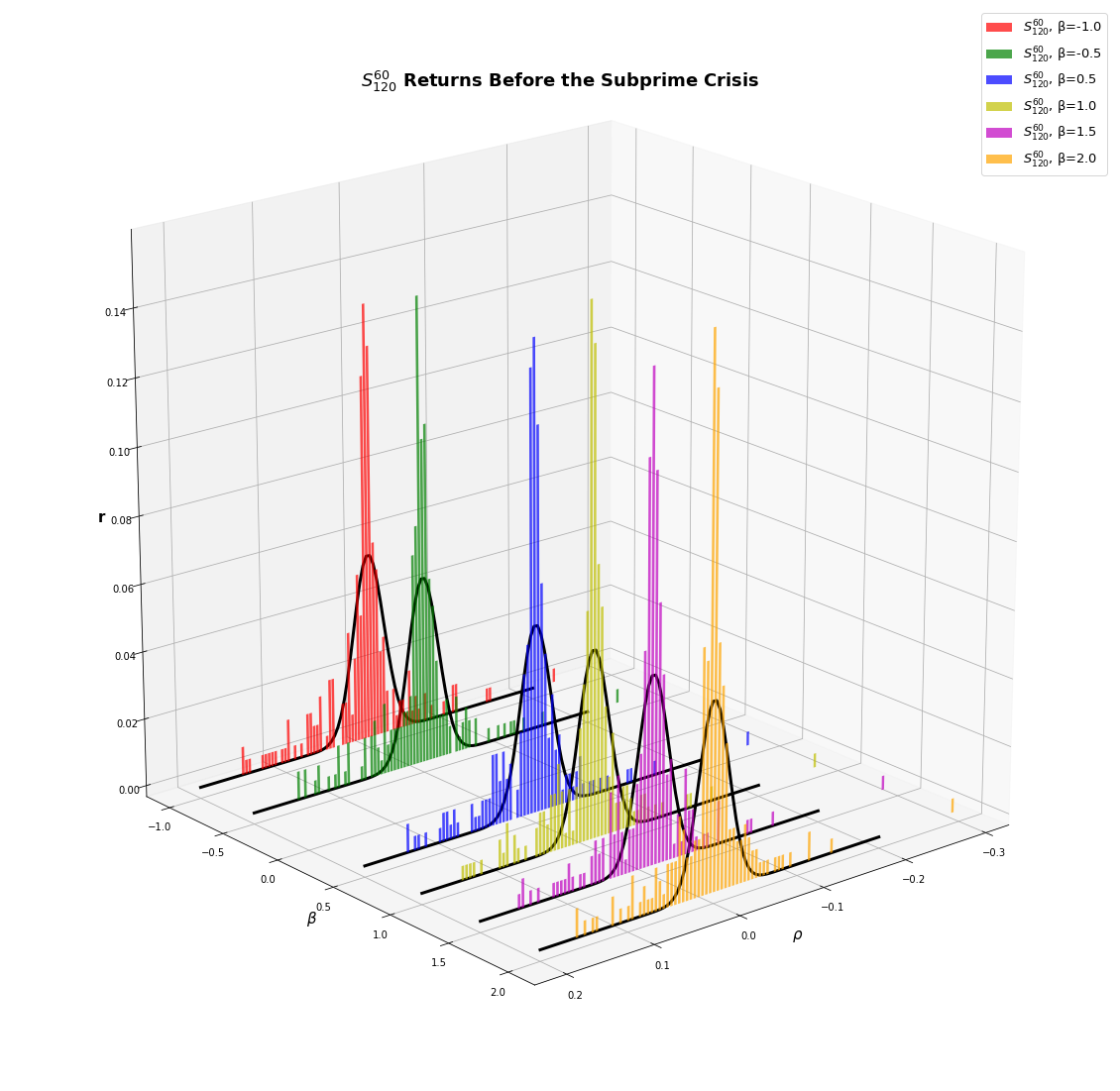
Fig. 13: The distribution of returns from the \(S_{120}^{60}\) investment strategy before the Subprime Crisis.
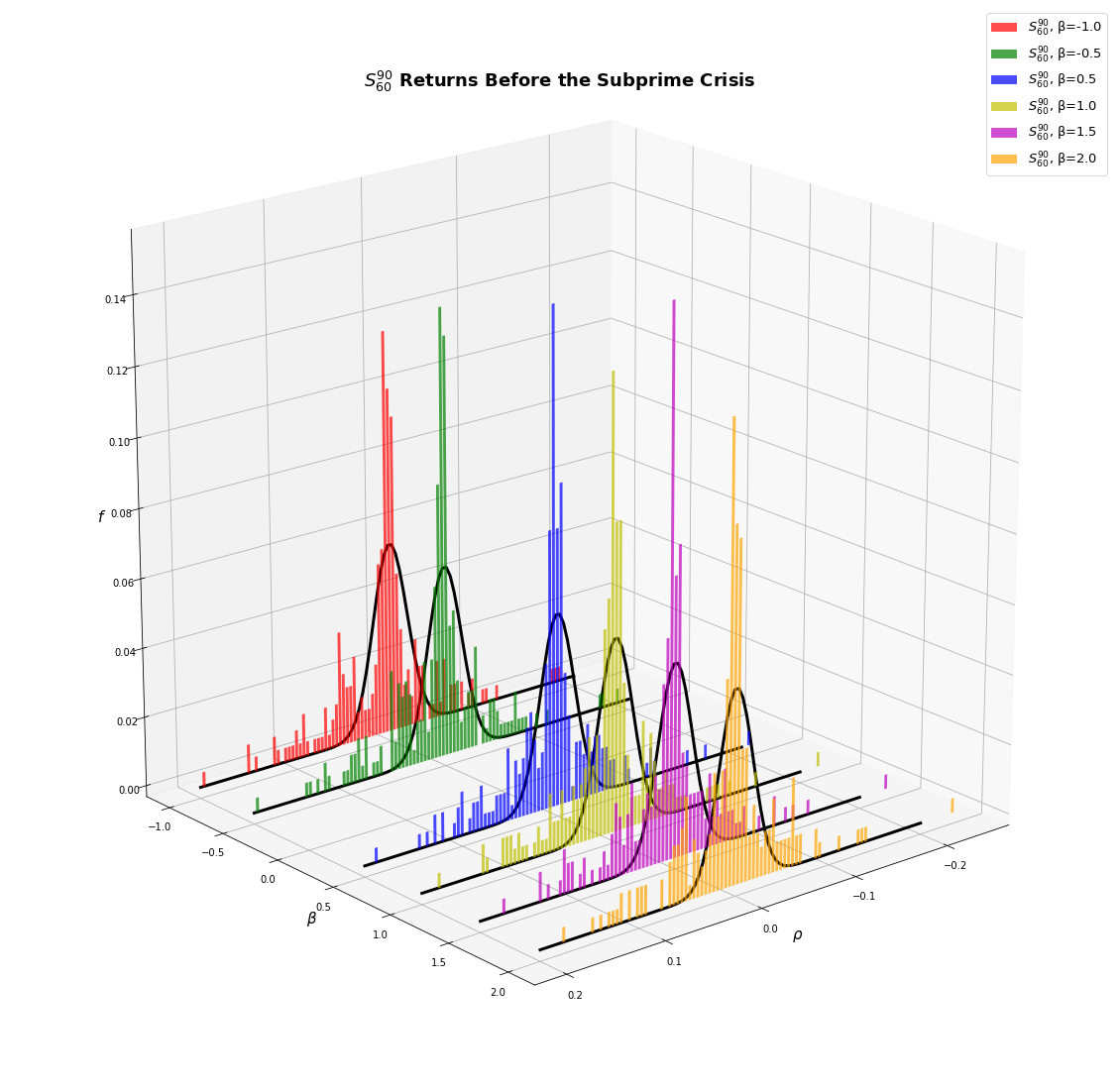
Fig. 14: The distribution of returns from the \(S_{60}^{90}\) investment strategy before the Subprime Crisis.
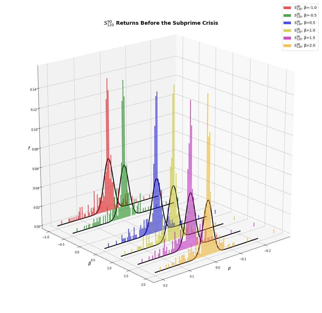
Fig. 15: The distribution of returns from the \(S_{120}^{90}\) investment strategy before the Subprime Crisis.
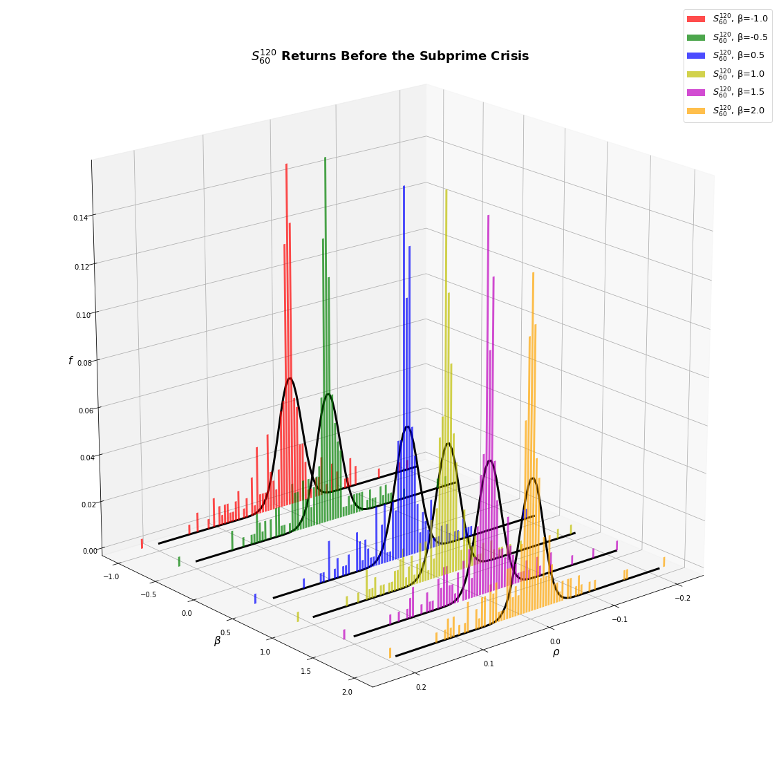
Fig. 16: The distribution of returns from the \(S_{120}^{60}\) investment strategy before the Subprime Crisis.
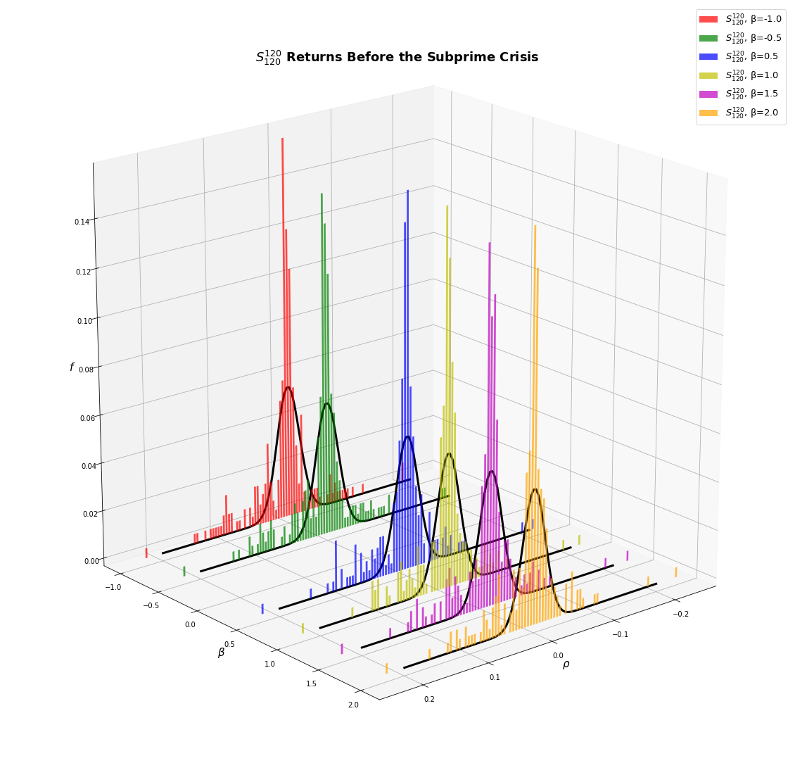
Fig. 17: The distribution of returns from the \(S_{120}^{120}\) investment strategy before the Subprime Crisis.
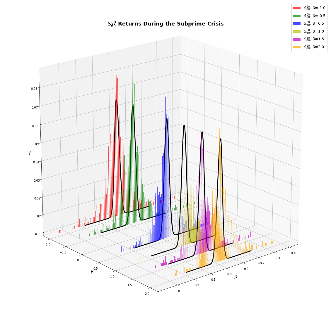
Fig. 18: The distribution of returns from the \(S_{60}^{60}\) investment strategy during the Subprime Crisis.
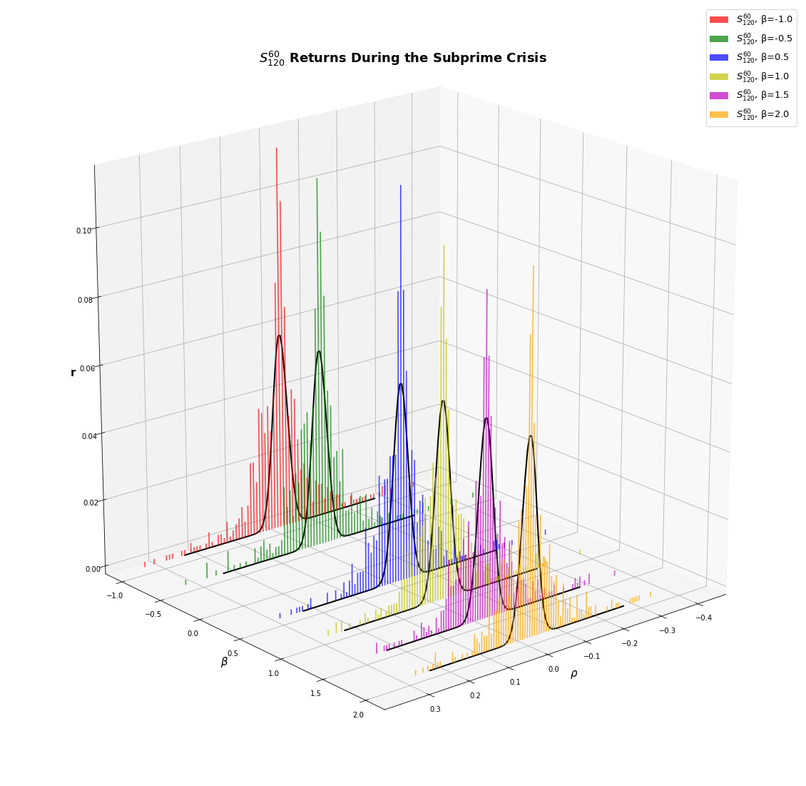
Fig. 19: The distribution of returns from the \(S_{120}^{60}\) investment strategy during the Subprime Crisis.

Fig. 20: The distribution of returns from the \(S_{60}^{90}\) investment strategy during the Subprime Crisis.

Fig. 21: The distribution of returns from the \(S_{120}^{60}\) investment strategy during the Subprime Crisis.

Fig. 22: The distribution of returns from the \(S_{60}^{120}\) investment strategy during the Subprime Crisis.
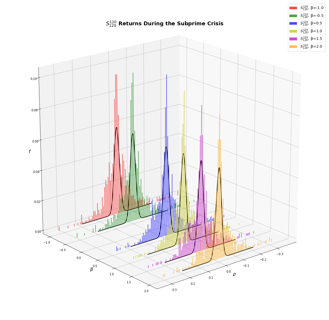
Fig. 23: The distribution of returns from the \(S_{120}^{120}\) investment strategy during the Subprime Crisis.

Fig. 24: The distribution of returns from the \(S_{60}^{60}\) investment strategy after the Subprime Crisis.
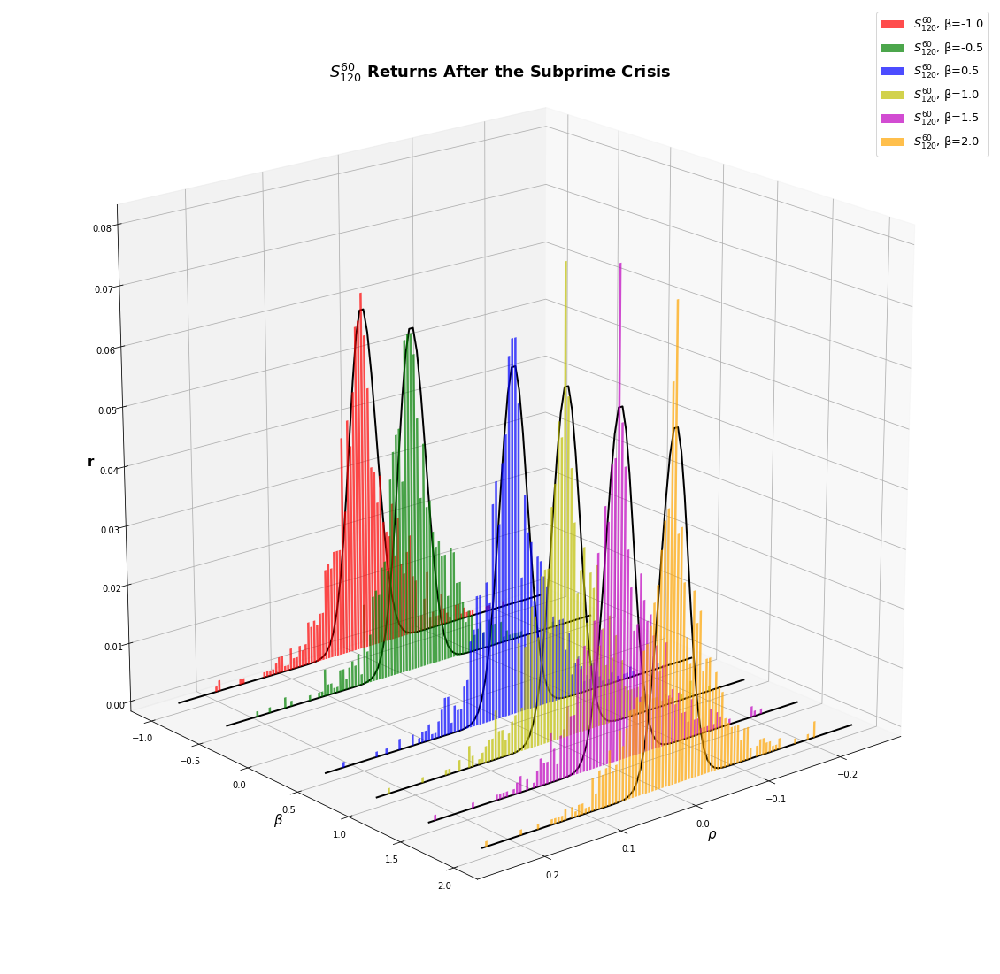
Fig. 25: The distribution of returns from the \(S_{120}^{60}\) investment strategy after the Subprime Crisis.
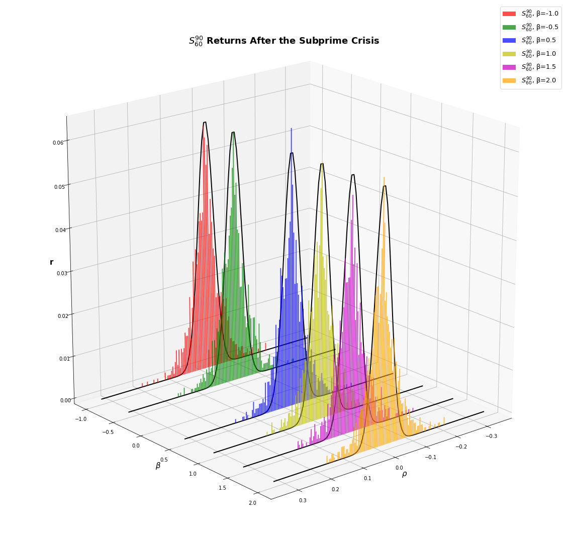
Fig. 26: The distribution of returns from the \(S_{60}^{90}\) investment strategy after the Subprime Crisis.

Fig. 27: The distribution of returns from the \(S_{120}^{90}\) investment strategy after the Subprime Crisis.
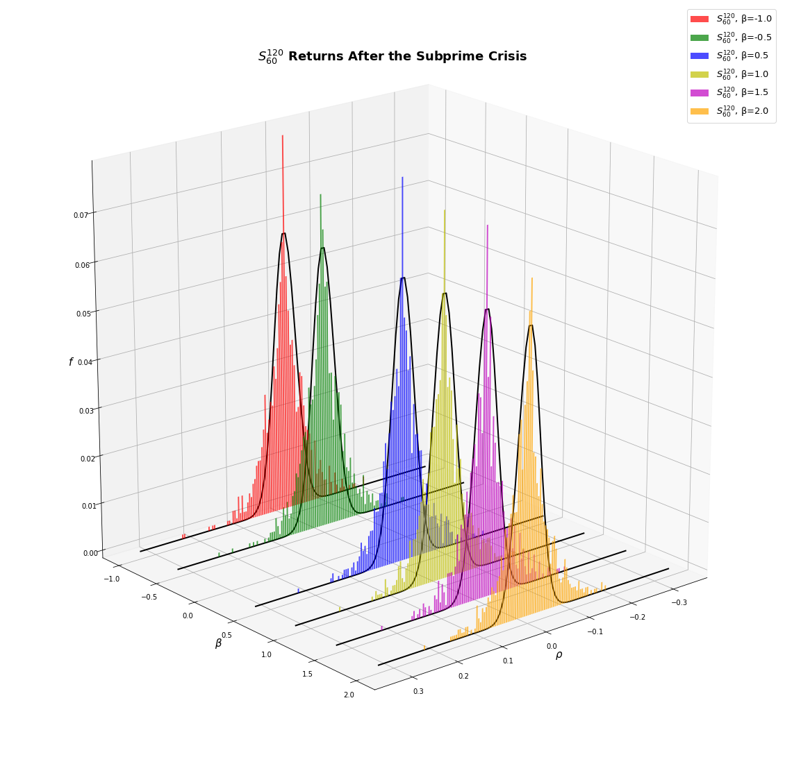
Fig. 28: The distribution of returns from the \(S_{60}^{120}\) investment strategy after the Subprime Crisis.
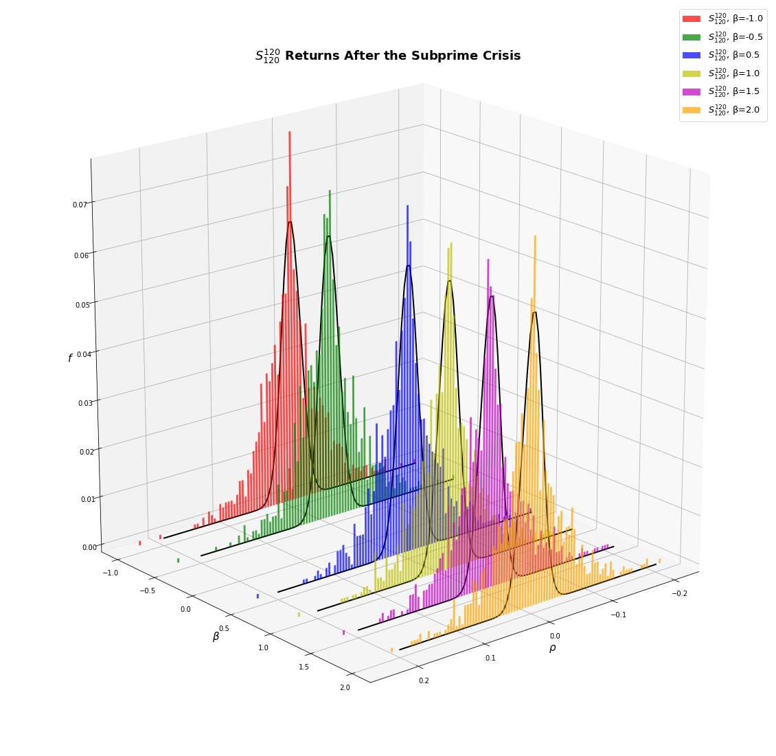
Fig. 29: The distribution of returns from the \(S_{120}^{120}\) investment strategy after the Subprime Crisis.

Fig. 30: The distribution of returns from the \(S_{60}^{60}\) investment strategy before COVID-19.
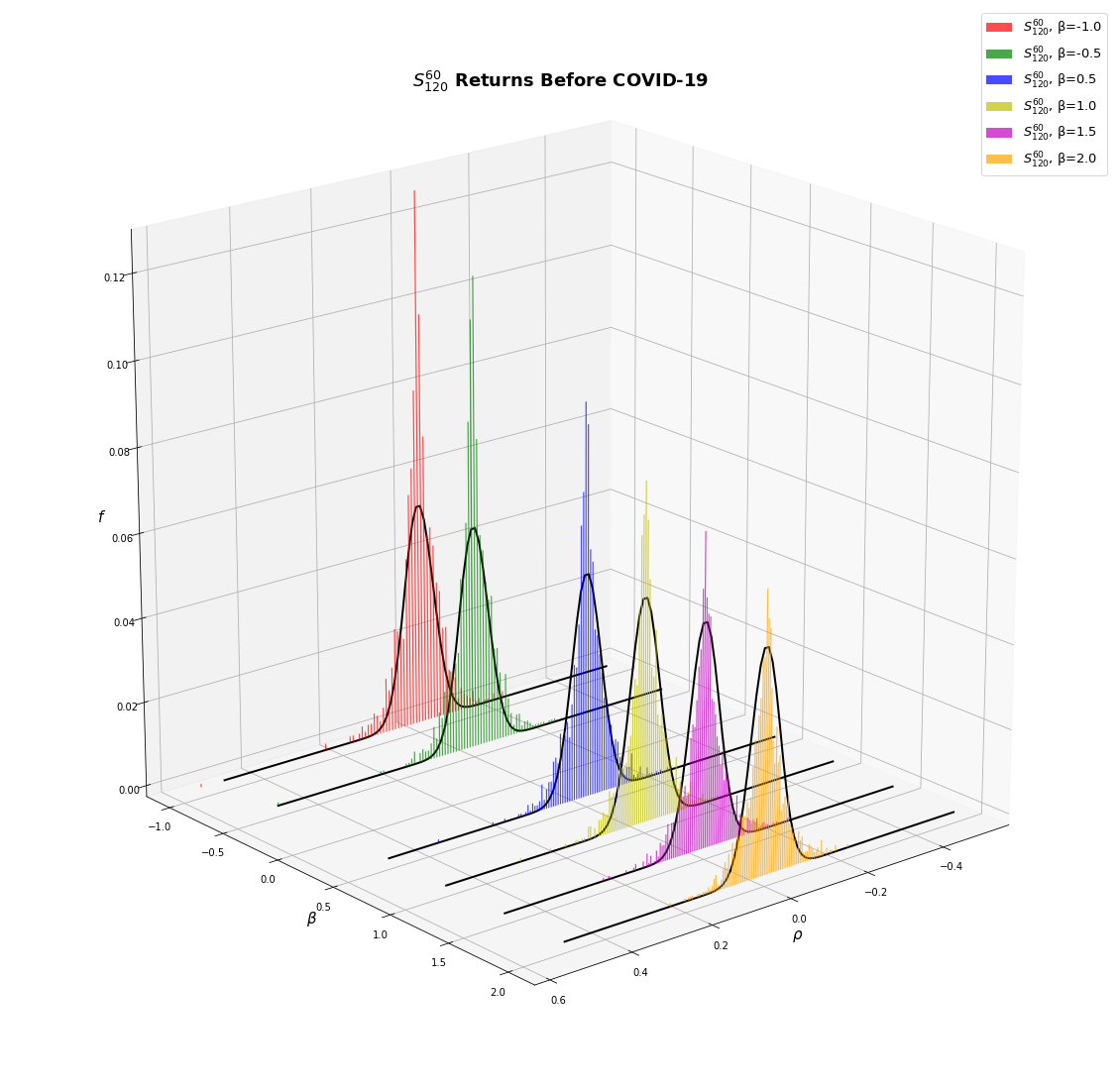
Fig. 31: The distribution of returns from the \(S_{120}^{60}\) investment strategy before COVID-19.
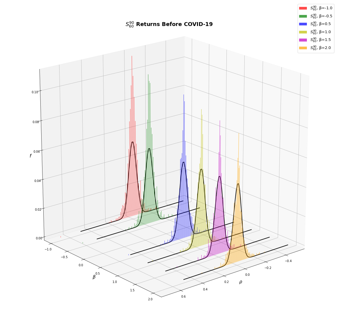
Fig. 32: The distribution of returns from the \(S_{60}^{90}\) investment strategy before COVID-19.
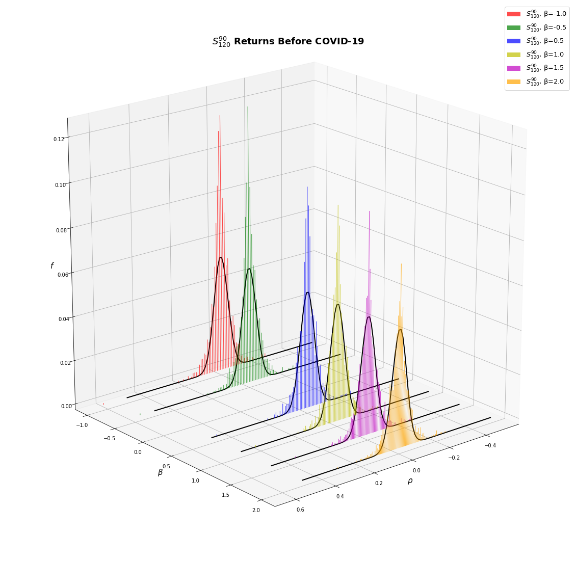
Fig. 33: The distribution of returns from the \(S_{120}^{90}\) investment strategy before COVID-19.
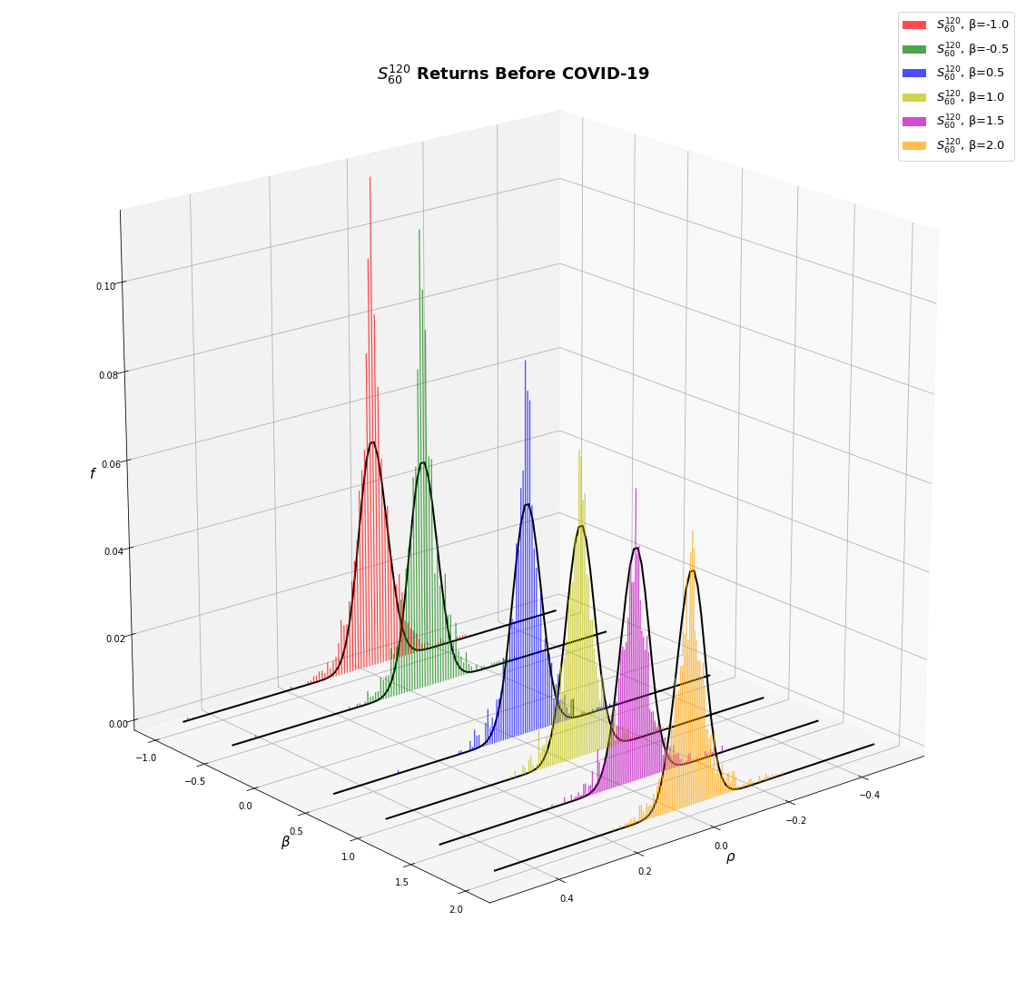
Fig. 34: The distribution of returns from the \(S_{60}^{120}\) investment strategy before COVID-19.

Fig. 35: The distribution of returns from the \(S_{120}^{120}\) investment strategy before COVID-19.
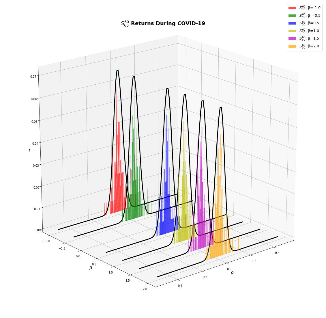
Fig. 36: The distribution of returns from the \(S_{60}^{60}\) investment strategy during COVID-19.
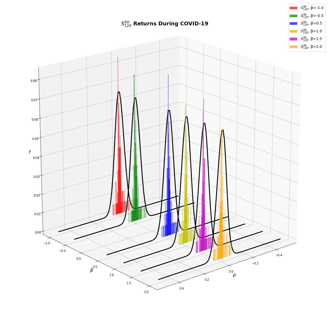
Fig. 37: The distribution of returns from the \(S_{120}^{60}\) investment strategy during COVID-19.
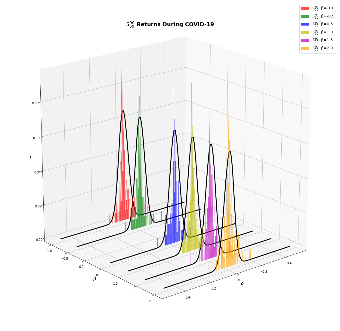
Fig. 38: The distribution of returns from the \(S_{60}^{90}\) investment strategy during COVID-19.
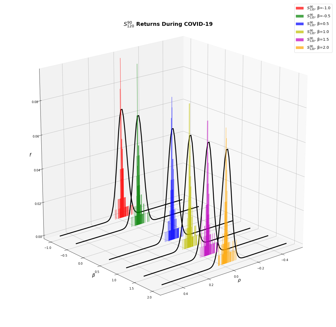
Fig. 39: The distribution of returns from the \(S_{120}^{90}\) investment strategy during COVID-19.
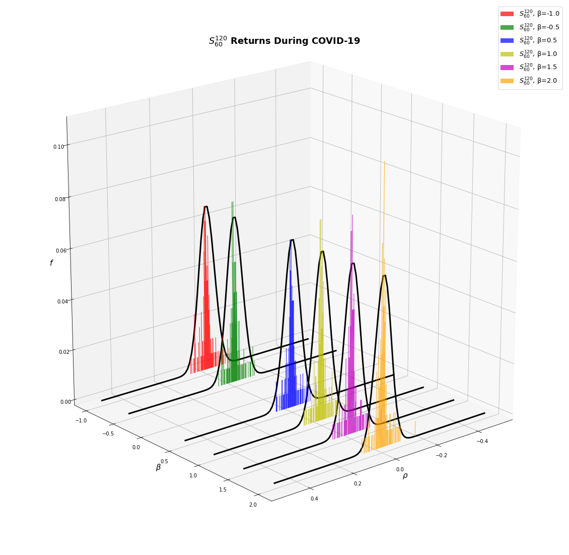
Fig. 40: The distribution of returns from the \(S_{60}^{120}\) investment strategy during COVID-19.
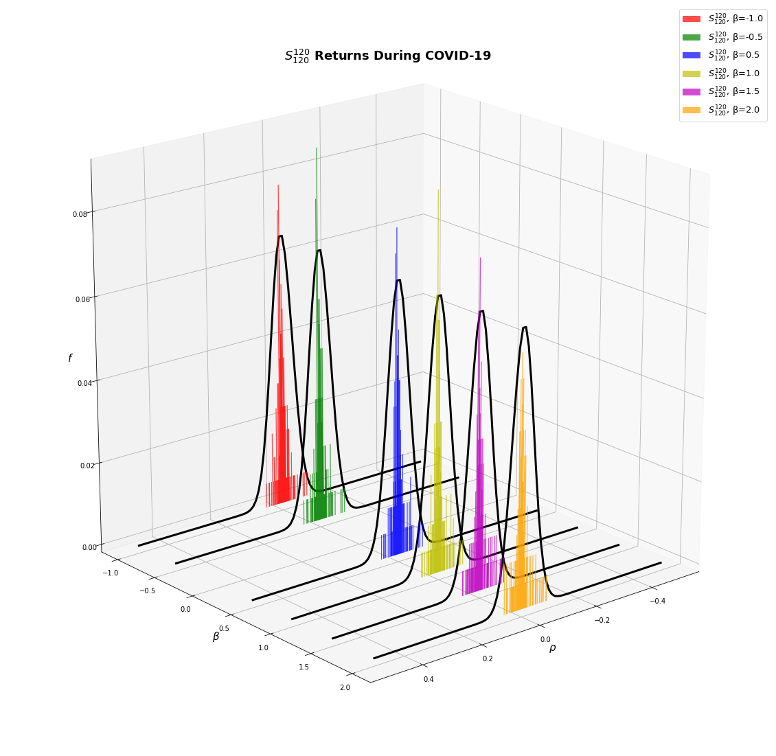
Fig. 41: The distribution of returns from the \(S_{120}^{120}\) investment strategy during COVID-19.
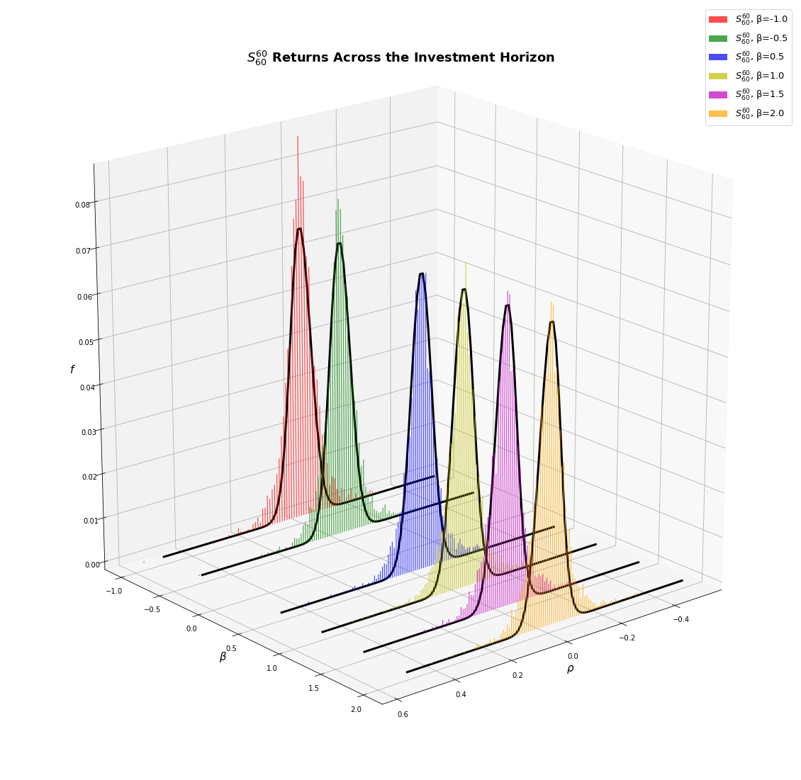
Fig. 42: The distribution of returns from the \(S_{60}^{60}\) investment strategy across the full investment horizon.

Fig. 43: The distribution of returns from the \(S_{120}^{60}\) investment strategy across the full investment horizon.
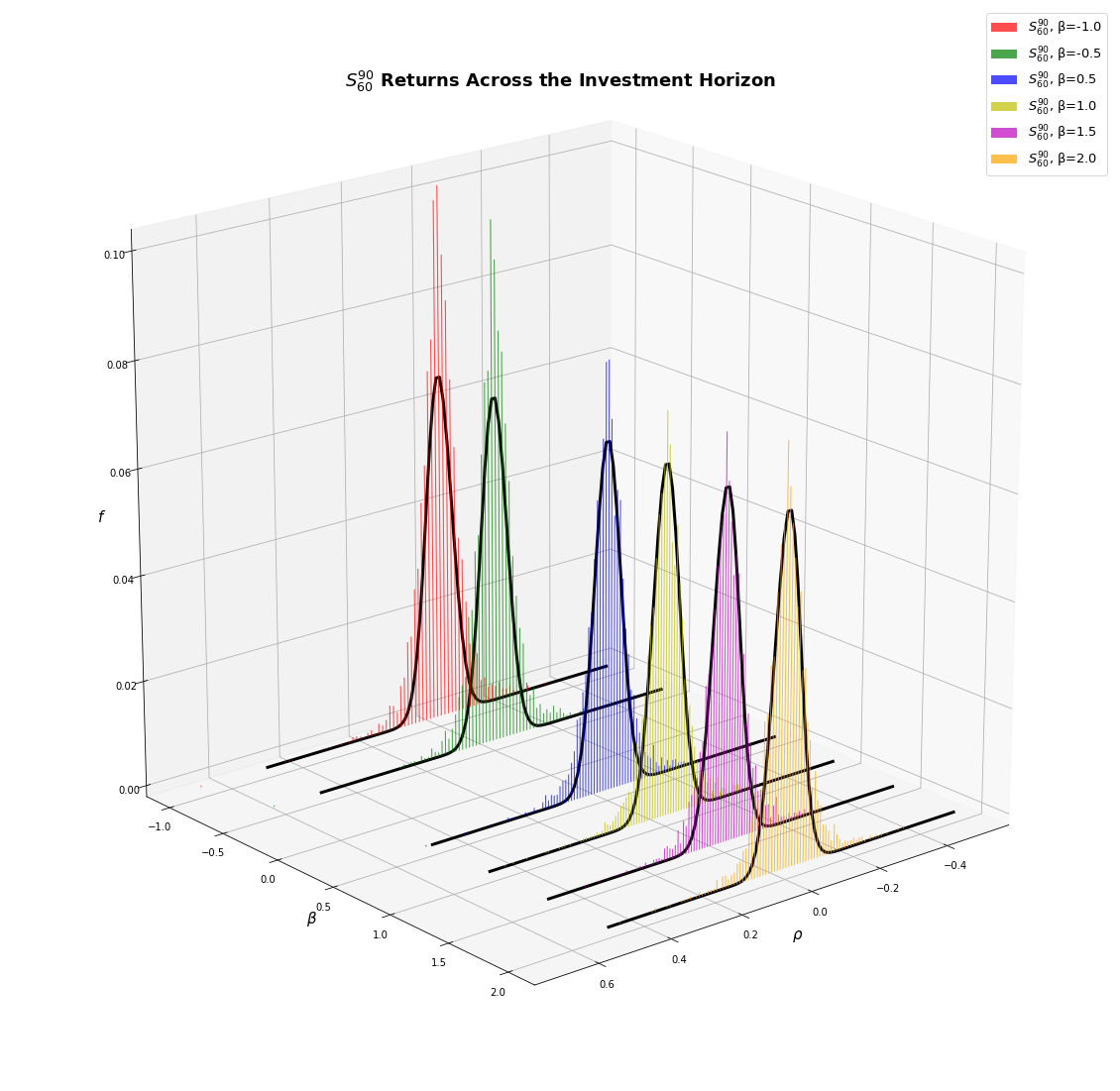
Fig. 44: The distribution of returns from the \(S_{60}^{90}\) investment strategy across the full investment horizon.
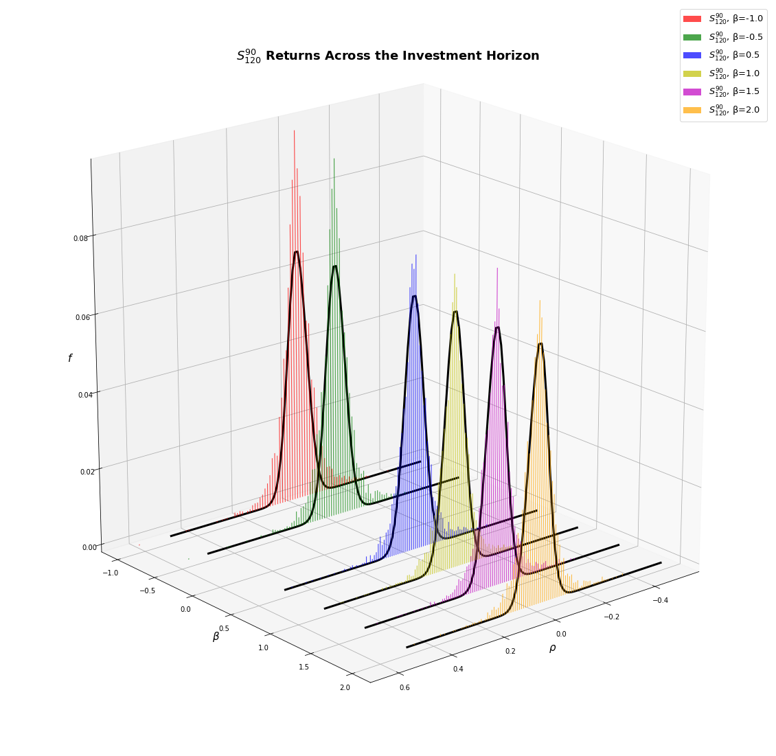
Fig. 45: The distribution of returns from the \(S_{120}^{90}\) investment strategy across the full investment horizon.
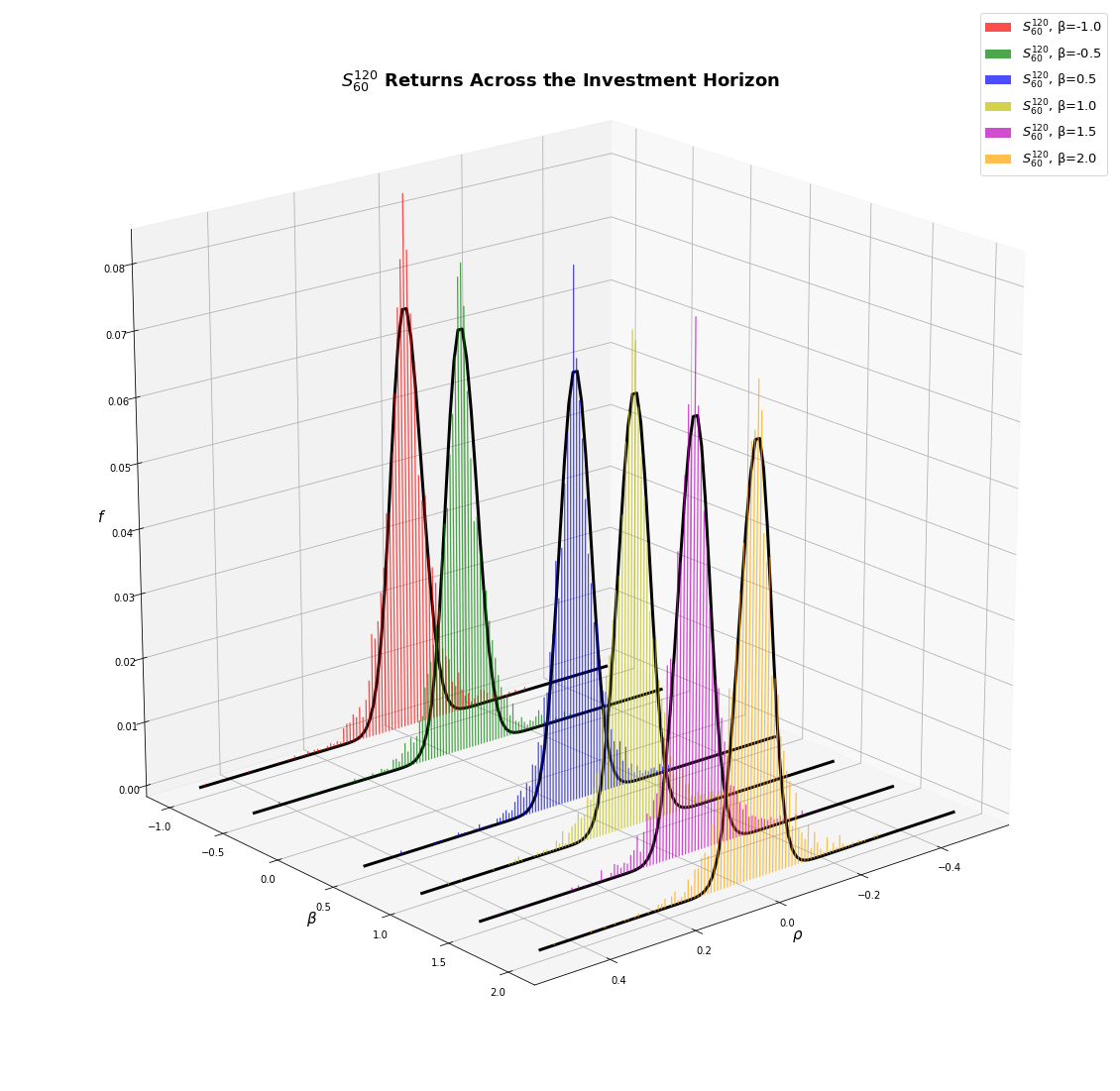
Fig. 46: The distribution of returns from the \(S_{60}^{120}\) investment strategy across the full investment horizon.
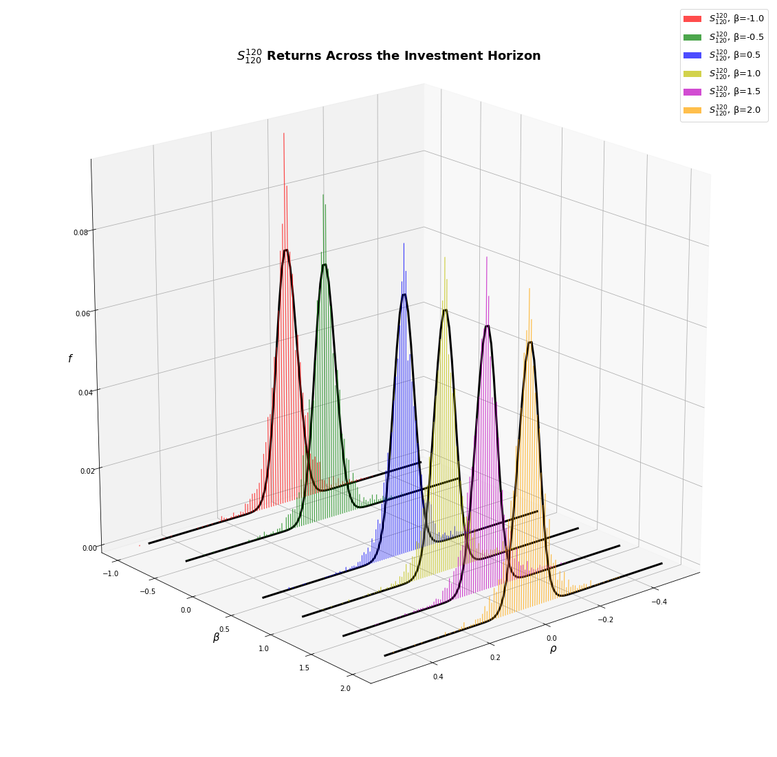
Fig. 47: The distribution of returns from the \(S_{120}^{120}\) investment strategy across the full investment horizon.
i. Before the Subprime Crisis
| \(S^{60}_{60}(\beta=-1.0)\) | \(S^{60}_{60}(\beta=-0.5)\) | \(S^{60}_{60}(\beta=0.5)\) | \(S^{60}_{60}(\beta=1.0)\) | \(S^{60}_{60}(\beta=1.5)\) | \(S^{60}_{60}(\beta=2.0)\) | \(S^{60}_{120}(\beta=-1.0)\) | \(S^{60}_{120}(\beta=-0.5)\) | \(S^{60}_{120}(\beta=0.5)\) | \(S^{60}_{120}(\beta=1.0)\) | \(S^{60}_{120}(\beta=1.5)\) | \(S^{60}_{120}(\beta=2.0)\) | \(S^{90}_{60}(\beta=-1.0)\) | \(S^{90}_{60}(\beta=-0.5)\) | \(S^{90}_{60}(\beta=0.5)\) | \(S^{90}_{60}(\beta=1.0)\) | \(S^{90}_{60}(\beta=1.5)\) | \(S^{90}_{60}(\beta=2.0)\) | \(S^{90}_{120}(\beta=-1.0)\) | \(S^{90}_{120}(\beta=-0.5)\) | \(S^{90}_{120}(\beta=0.5)\) | \(S^{90}_{120}(\beta=1.0)\) | \(S^{90}_{120}(\beta=1.5)\) | \(S^{90}_{120}(\beta=2.0)\) | \(S^{120}_{60}(\beta=-1.0)\) | \(S^{120}_{60}(\beta=-0.5)\) | \(S^{120}_{60}(\beta=0.5)\) | \(S^{120}_{60}(\beta=1.0)\) | \(S^{120}_{60}(\beta=1.5)\) | \(S^{120}_{60}(\beta=2.0)\) | \(S^{120}_{120}(\beta=-1.0)\) | \(S^{120}_{120}(\beta=-0.5)\) | \(S^{120}_{120}(\beta=0.5)\) | \(S^{120}_{120}(\beta=1.0)\) | \(S^{120}_{120}(\beta=1.5)\) | \(S^{120}_{120}(\beta=2.0)\) | SPY | |
|---|---|---|---|---|---|---|---|---|---|---|---|---|---|---|---|---|---|---|---|---|---|---|---|---|---|---|---|---|---|---|---|---|---|---|---|---|---|
| Cumulative Returns (Annual) | 3.8368 | 3.8297 | 3.8219 | 3.7803 | 3.6472 | 3.4493 | 4.9195 | 4.8497 | 4.5314 | 4.3239 | 4.0830 | 3.8720 | 5.9865 | 5.9496 | 5.5748 | 5.2739 | 5.0177 | 4.9510 | 6.7861 | 6.5281 | 5.9731 | 5.7247 | 5.5887 | 5.3392 | 6.6619 | 6.2123 | 5.6994 | 5.4030 | 4.9486 | 4.5644 | 6.1897 | 5.8874 | 5.2227 | 4.9259 | 4.7650 | 4.5420 | 0.9644 |
| Arithmetic Mean Returns (Annual) | 1.6503 | 1.6345 | 1.6235 | 1.6178 | 1.5910 | 1.5496 | 1.8661 | 1.8365 | 1.7557 | 1.7112 | 1.6609 | 1.6191 | 2.1038 | 2.0845 | 2.0043 | 1.9482 | 1.9039 | 1.9036 | 2.2063 | 2.1534 | 2.0526 | 2.0112 | 1.9937 | 1.9551 | 2.1951 | 2.1020 | 2.0001 | 1.9401 | 1.8488 | 1.7693 | 2.1117 | 2.0423 | 1.9017 | 1.8435 | 1.8185 | 1.7805 | -0.0214 |
| Geometric Mean Returns (Annual) | 1.3483 | 1.3464 | 1.3443 | 1.3333 | 1.2973 | 1.2412 | 1.5983 | 1.5839 | 1.5156 | 1.4684 | 1.4108 | 1.3574 | 1.7959 | 1.7897 | 1.7242 | 1.6683 | 1.6182 | 1.6047 | 1.9222 | 1.8832 | 1.7937 | 1.7509 | 1.7267 | 1.6807 | 1.9036 | 1.8332 | 1.7464 | 1.6927 | 1.6042 | 1.5229 | 1.8295 | 1.7791 | 1.6585 | 1.5996 | 1.5662 | 1.5180 | -0.0362 |
| Minimum Return (Annual) | -44.7289 | -47.4883 | -52.9759 | -56.1288 | -59.1416 | -62.2160 | -57.1246 | -59.9001 | -65.3671 | -68.0963 | -70.7905 | -73.5078 | -46.2963 | -47.3185 | -52.4121 | -55.4892 | -57.7419 | -59.3230 | -52.7134 | -54.9567 | -59.8627 | -62.2949 | -64.8629 | -67.3731 | -46.6696 | -46.6517 | -47.5185 | -49.0611 | -50.8233 | -52.6881 | -47.4232 | -48.8173 | -51.9945 | -54.1730 | -56.6386 | -58.8764 | -7.4084 |
| Max 10-day Drawdown | -0.3799 | -0.3683 | -0.3461 | -0.3564 | -0.3670 | -0.3768 | -0.3850 | -0.3759 | -0.4001 | -0.4169 | -0.4329 | -0.4425 | -0.3398 | -0.3132 | -0.2653 | -0.2688 | -0.2790 | -0.2930 | -0.3290 | -0.3162 | -0.2874 | -0.2732 | -0.2891 | -0.3101 | -0.3241 | -0.3006 | -0.2632 | -0.2491 | -0.2359 | -0.2286 | -0.3229 | -0.3080 | -0.2791 | -0.2648 | -0.2564 | -0.2616 | -0.0748 |
| Volatility | 0.7760 | 0.7583 | 0.7470 | 0.7536 | 0.7647 | 0.7819 | 0.7299 | 0.7082 | 0.6880 | 0.6904 | 0.6992 | 0.7138 | 0.7844 | 0.7681 | 0.7486 | 0.7474 | 0.7542 | 0.7705 | 0.7559 | 0.7370 | 0.7200 | 0.7210 | 0.7291 | 0.7377 | 0.7668 | 0.7366 | 0.7158 | 0.7071 | 0.7020 | 0.7035 | 0.7543 | 0.7286 | 0.6999 | 0.7001 | 0.7117 | 0.7251 | 0.1723 |
| Sharpe Ratio (Annual) | 2.0495 | 2.0763 | 2.0931 | 2.0670 | 2.0021 | 1.9051 | 2.4744 | 2.5083 | 2.4647 | 2.3918 | 2.2896 | 2.1842 | 2.6055 | 2.6359 | 2.5971 | 2.5263 | 2.4450 | 2.3928 | 2.8394 | 2.8406 | 2.7674 | 2.7063 | 2.6521 | 2.5691 | 2.7844 | 2.7721 | 2.7102 | 2.6588 | 2.5480 | 2.4298 | 2.7198 | 2.7206 | 2.6316 | 2.5474 | 2.4710 | 2.3728 | -0.4722 |
| Kurtosis (Annual) | 2.5804 | 2.8307 | 3.3305 | 3.5849 | 3.7634 | 3.8714 | 4.4851 | 5.4319 | 7.6044 | 8.5310 | 9.2204 | 9.5967 | 3.0385 | 3.2162 | 3.4069 | 3.5860 | 3.6444 | 3.6409 | 3.9851 | 4.5576 | 5.7836 | 6.2730 | 6.5307 | 6.7731 | 3.8053 | 4.2873 | 5.2117 | 5.3481 | 5.2687 | 5.2129 | 4.3542 | 5.0143 | 6.2790 | 6.6741 | 6.9157 | 6.7475 | 0.4725 |
| Skew (Annual) | -0.1125 | -0.0674 | -0.0141 | -0.0263 | -0.0899 | -0.1957 | -0.1572 | -0.1974 | -0.3666 | -0.4649 | -0.5588 | -0.6417 | -0.0644 | -0.0298 | -0.0231 | -0.0875 | -0.1587 | -0.2063 | 0.1418 | 0.1389 | 0.0700 | 0.0073 | -0.0626 | -0.1679 | 0.2228 | 0.2654 | 0.3314 | 0.3460 | 0.2738 | 0.1673 | 0.2465 | 0.2730 | 0.2700 | 0.2304 | 0.2082 | 0.1426 | -0.2775 |
| mVaR (Annual) | -115.6217 | -111.5075 | -107.8824 | -108.8420 | -111.8536 | -116.9951 | -104.8767 | -101.0395 | -98.4963 | -99.6899 | -102.1890 | -105.8134 | -112.3369 | -108.8135 | -105.8078 | -107.0607 | -109.8252 | -113.4892 | -101.2292 | -97.8880 | -95.6079 | -96.5976 | -99.0002 | -102.3677 | -101.4282 | -95.8436 | -90.6748 | -89.2950 | -90.7552 | -93.7379 | -98.7224 | -93.8034 | -88.7535 | -89.4146 | -91.3533 | -95.1656 | -29.6452 |
| VaR (Daily) | -7.4123 | -7.2348 | -7.1217 | -7.1931 | -7.3186 | -7.5142 | -6.8466 | -6.6332 | -6.4548 | -6.4973 | -6.6094 | -6.7780 | -7.3185 | -7.1562 | -6.9863 | -6.9963 | -7.0838 | -7.2539 | -6.9812 | -6.8053 | -6.6693 | -6.6961 | -6.7874 | -6.8918 | -7.0990 | -6.8224 | -6.6468 | -6.5802 | -6.5638 | -6.6105 | -7.0027 | -6.7630 | -6.5199 | -6.5459 | -6.6760 | -6.8309 | -1.8009 |
| VaR (Annual) | -117.1987 | -114.3926 | -112.6036 | -113.7322 | -115.7177 | -118.8103 | -108.2549 | -104.8806 | -102.0586 | -102.7318 | -104.5033 | -107.1703 | -115.7161 | -113.1498 | -110.4633 | -110.6212 | -112.0051 | -114.6945 | -110.3832 | -107.6020 | -105.4506 | -105.8750 | -107.3183 | -108.9685 | -112.2452 | -107.8721 | -105.0946 | -104.0414 | -103.7827 | -104.5208 | -110.7230 | -106.9332 | -103.0889 | -103.5005 | -105.5560 | -108.0065 | -28.4753 |
| CVaR (Annual) | -178.6040 | -173.1223 | -165.8598 | -164.1459 | -164.8841 | -168.8750 | -169.0285 | -160.1094 | -150.8754 | -151.0805 | -154.0041 | -160.9780 | -175.3734 | -169.5929 | -163.5622 | -163.7087 | -166.0813 | -168.4409 | -163.7402 | -156.3287 | -146.7029 | -147.0361 | -148.4515 | -152.5007 | -172.6897 | -162.8454 | -156.2081 | -152.0010 | -151.9953 | -154.3195 | -165.9046 | -157.0280 | -145.9796 | -146.2212 | -150.0774 | -154.9998 | -40.1797 |
ii. During the Subrime Crisis
| \(S^{60}_{60}(\beta=-1.0)\) | \(S^{60}_{60}(\beta=-0.5)\) | \(S^{60}_{60}(\beta=0.5)\) | \(S^{60}_{60}(\beta=1.0)\) | \(S^{60}_{60}(\beta=1.5)\) | \(S^{60}_{60}(\beta=2.0)\) | \(S^{60}_{120}(\beta=-1.0)\) | \(S^{60}_{120}(\beta=-0.5)\) | \(S^{60}_{120}(\beta=0.5)\) | \(S^{60}_{120}(\beta=1.0)\) | \(S^{60}_{120}(\beta=1.5)\) | \(S^{60}_{120}(\beta=2.0)\) | \(S^{90}_{60}(\beta=-1.0)\) | \(S^{90}_{60}(\beta=-0.5)\) | \(S^{90}_{60}(\beta=0.5)\) | \(S^{90}_{60}(\beta=1.0)\) | \(S^{90}_{60}(\beta=1.5)\) | \(S^{90}_{60}(\beta=2.0)\) | \(S^{90}_{120}(\beta=-1.0)\) | \(S^{90}_{120}(\beta=-0.5)\) | \(S^{90}_{120}(\beta=0.5)\) | \(S^{90}_{120}(\beta=1.0)\) | \(S^{90}_{120}(\beta=1.5)\) | \(S^{90}_{120}(\beta=2.0)\) | \(S^{120}_{60}(\beta=-1.0)\) | \(S^{120}_{60}(\beta=-0.5)\) | \(S^{120}_{60}(\beta=0.5)\) | \(S^{120}_{60}(\beta=1.0)\) | \(S^{120}_{60}(\beta=1.5)\) | \(S^{120}_{60}(\beta=2.0)\) | \(S^{120}_{120}(\beta=-1.0)\) | \(S^{120}_{120}(\beta=-0.5)\) | \(S^{120}_{120}(\beta=0.5)\) | \(S^{120}_{120}(\beta=1.0)\) | \(S^{120}_{120}(\beta=1.5)\) | \(S^{120}_{120}(\beta=2.0)\) | SPY | |
|---|---|---|---|---|---|---|---|---|---|---|---|---|---|---|---|---|---|---|---|---|---|---|---|---|---|---|---|---|---|---|---|---|---|---|---|---|---|
| Cumulative Returns (Annual) | 0.5758 | 0.6588 | 0.8186 | 0.8525 | 0.8595 | 0.8314 | 0.5168 | 0.5640 | 0.6990 | 0.7558 | 0.8134 | 0.8153 | 0.4492 | 0.5626 | 0.7766 | 0.8633 | 0.9115 | 0.9357 | 0.4357 | 0.5282 | 0.7310 | 0.7529 | 0.7788 | 0.7837 | 0.3731 | 0.4459 | 0.5725 | 0.6234 | 0.6465 | 0.6525 | 0.4256 | 0.5423 | 0.7528 | 0.8237 | 0.8527 | 0.8456 | 0.9407 |
| Arithmetic Mean Returns (Annual) | 0.2964 | 0.3602 | 0.5012 | 0.5420 | 0.5756 | 0.5971 | 0.1600 | 0.1828 | 0.3075 | 0.3767 | 0.4555 | 0.4865 | -0.0260 | 0.1347 | 0.4196 | 0.5403 | 0.6335 | 0.7144 | 0.0189 | 0.1507 | 0.3806 | 0.3990 | 0.4410 | 0.4767 | -0.3405 | -0.1973 | 0.0230 | 0.1211 | 0.1881 | 0.2487 | -0.1044 | 0.0902 | 0.3559 | 0.4419 | 0.4895 | 0.5154 | -0.0094 |
| Geometric Mean Returns (Annual) | -0.5514 | -0.4169 | -0.2001 | -0.1595 | -0.1514 | -0.1845 | -0.6592 | -0.5720 | -0.3579 | -0.2798 | -0.2064 | -0.2041 | -0.7991 | -0.5745 | -0.2527 | -0.1469 | -0.0927 | -0.0665 | -0.8295 | -0.6375 | -0.3131 | -0.2836 | -0.2498 | -0.2436 | -0.9840 | -0.8064 | -0.5572 | -0.4721 | -0.4358 | -0.4265 | -0.8528 | -0.6112 | -0.2838 | -0.1939 | -0.1593 | -0.1676 | -0.0611 |
| Minimum Return (Annual) | -100.5287 | -99.1987 | -91.0196 | -84.5105 | -78.7393 | -85.6251 | -105.7245 | -104.0076 | -97.7272 | -92.6221 | -86.8214 | -81.5243 | -90.3795 | -83.4078 | -71.9763 | -69.0653 | -77.6938 | -85.9676 | -97.9859 | -98.3732 | -93.8185 | -89.1067 | -84.3366 | -79.7000 | -91.0885 | -81.1770 | -74.9677 | -71.0308 | -75.2545 | -82.7175 | -90.8029 | -90.8937 | -85.6258 | -82.2741 | -78.2641 | -78.2427 | -24.6119 |
| Max 10-day Drawdown | -0.6193 | -0.6213 | -0.6277 | -0.6362 | -0.6461 | -0.6591 | -0.6092 | -0.6104 | -0.6287 | -0.6404 | -0.6472 | -0.6588 | -0.6077 | -0.6093 | -0.6272 | -0.6370 | -0.6488 | -0.6620 | -0.6091 | -0.6105 | -0.6185 | -0.6313 | -0.6430 | -0.6548 | -0.5813 | -0.5757 | -0.6065 | -0.6214 | -0.6382 | -0.6552 | -0.5934 | -0.5930 | -0.6067 | -0.6193 | -0.6330 | -0.6474 | -0.2495 |
| Volatility | 1.2761 | 1.2223 | 1.1623 | 1.1639 | 1.1862 | 1.2313 | 1.2566 | 1.2058 | 1.1337 | 1.1273 | 1.1329 | 1.1583 | 1.2141 | 1.1673 | 1.1398 | 1.1533 | 1.1863 | 1.2314 | 1.2757 | 1.2313 | 1.1564 | 1.1475 | 1.1553 | 1.1809 | 1.1093 | 1.0836 | 1.0604 | 1.0730 | 1.1013 | 1.1467 | 1.1965 | 1.1614 | 1.1122 | 1.1095 | 1.1218 | 1.1519 | 0.3222 |
| Sharpe Ratio (Annual) | 0.1853 | 0.2456 | 0.3796 | 0.4141 | 0.4347 | 0.4362 | 0.0796 | 0.1019 | 0.2183 | 0.2810 | 0.3491 | 0.3682 | -0.0708 | 0.0640 | 0.3155 | 0.4165 | 0.4834 | 0.5315 | -0.0322 | 0.0736 | 0.2772 | 0.2954 | 0.3298 | 0.3528 | -0.3610 | -0.2375 | -0.0349 | 0.0570 | 0.1163 | 0.1646 | -0.1374 | 0.0260 | 0.2660 | 0.3442 | 0.3829 | 0.3953 | -0.2154 |
| Kurtosis (Annual) | 4.4841 | 4.3579 | 3.6133 | 3.1531 | 2.9214 | 3.0115 | 4.9096 | 5.1694 | 4.6879 | 4.1765 | 3.6973 | 3.4233 | 4.1680 | 3.6251 | 2.8308 | 2.5706 | 2.4056 | 2.3761 | 4.0819 | 4.1152 | 3.8520 | 3.6036 | 3.3220 | 3.1427 | 4.3959 | 4.0773 | 3.5580 | 3.3767 | 3.2577 | 3.2639 | 4.5464 | 4.3383 | 3.9114 | 3.6465 | 3.4129 | 3.2665 | 7.8228 |
| Skew (Annual) | -0.3124 | -0.3596 | -0.4432 | -0.4257 | -0.3769 | -0.2913 | -0.2235 | -0.2713 | -0.3288 | -0.3345 | -0.3314 | -0.2899 | -0.5125 | -0.4630 | -0.4429 | -0.4282 | -0.3861 | -0.3204 | -0.3489 | -0.3413 | -0.4078 | -0.4238 | -0.4043 | -0.3501 | -0.5355 | -0.4285 | -0.3866 | -0.3603 | -0.3131 | -0.2435 | -0.4393 | -0.4044 | -0.3865 | -0.3851 | -0.3591 | -0.3060 | 0.3943 |
| mVaR (Annual) | -207.5827 | -200.2151 | -193.7452 | -194.2999 | -196.8669 | -201.2673 | -201.1020 | -193.7299 | -184.1811 | -184.0272 | -185.4440 | -188.8037 | -206.7435 | -197.5074 | -192.2492 | -193.9383 | -198.0556 | -203.0976 | -211.5567 | -203.0360 | -191.8636 | -191.3095 | -192.4147 | -195.2213 | -191.0681 | -183.3897 | -178.0079 | -179.1400 | -182.3161 | -187.2965 | -201.0031 | -193.2848 | -183.8202 | -183.3809 | -184.8708 | -188.4372 | -44.2700 |
| VaR (Daily) | -13.1571 | -12.5712 | -11.8907 | -11.8913 | -12.1096 | -12.5700 | -13.0088 | -12.4705 | -11.6713 | -11.5768 | -11.6030 | -11.8549 | -12.6406 | -12.0896 | -11.6897 | -11.7815 | -12.0879 | -12.5243 | -13.2630 | -12.7493 | -11.8780 | -11.7775 | -11.8419 | -12.0945 | -11.6763 | -11.3514 | -11.0216 | -11.1137 | -11.3815 | -11.8295 | -12.4893 | -12.0456 | -11.4279 | -11.3658 | -11.4740 | -11.7772 | -3.3560 |
| VaR (Annual) | -208.0315 | -198.7676 | -188.0077 | -188.0178 | -191.4688 | -198.7499 | -205.6869 | -197.1760 | -184.5397 | -183.0458 | -183.4596 | -187.4427 | -199.8661 | -191.1537 | -184.8310 | -186.2815 | -191.1263 | -198.0261 | -209.7064 | -201.5836 | -187.8076 | -186.2191 | -187.2369 | -191.2305 | -184.6192 | -179.4813 | -174.2668 | -175.7232 | -179.9566 | -187.0408 | -197.4733 | -190.4578 | -180.6912 | -179.7090 | -181.4191 | -186.2134 | -53.0626 |
| CVaR (Annual) | -325.7535 | -310.0824 | -297.5279 | -296.4889 | -297.7260 | -302.8519 | -320.9846 | -306.3446 | -287.7955 | -286.7799 | -287.6184 | -290.7606 | -314.6274 | -300.8983 | -291.9374 | -292.1202 | -295.2706 | -299.2538 | -329.8680 | -314.4450 | -297.8577 | -296.5007 | -295.4362 | -297.6577 | -293.3791 | -285.4468 | -274.2005 | -275.1119 | -280.0214 | -285.6853 | -316.2025 | -303.1984 | -287.6735 | -284.2934 | -284.2472 | -288.3882 | -77.6516 |
iii. After the Subprime Crisis
| \(S^{60}_{60}(\beta=-1.0)\) | \(S^{60}_{60}(\beta=-0.5)\) | \(S^{60}_{60}(\beta=0.5)\) | \(S^{60}_{60}(\beta=1.0)\) | \(S^{60}_{60}(\beta=1.5)\) | \(S^{60}_{60}(\beta=2.0)\) | \(S^{60}_{120}(\beta=-1.0)\) | \(S^{60}_{120}(\beta=-0.5)\) | \(S^{60}_{120}(\beta=0.5)\) | \(S^{60}_{120}(\beta=1.0)\) | \(S^{60}_{120}(\beta=1.5)\) | \(S^{60}_{120}(\beta=2.0)\) | \(S^{90}_{60}(\beta=-1.0)\) | \(S^{90}_{60}(\beta=-0.5)\) | \(S^{90}_{60}(\beta=0.5)\) | \(S^{90}_{60}(\beta=1.0)\) | \(S^{90}_{60}(\beta=1.5)\) | \(S^{90}_{60}(\beta=2.0)\) | \(S^{90}_{120}(\beta=-1.0)\) | \(S^{90}_{120}(\beta=-0.5)\) | \(S^{90}_{120}(\beta=0.5)\) | \(S^{90}_{120}(\beta=1.0)\) | \(S^{90}_{120}(\beta=1.5)\) | \(S^{90}_{120}(\beta=2.0)\) | \(S^{120}_{60}(\beta=-1.0)\) | \(S^{120}_{60}(\beta=-0.5)\) | \(S^{120}_{60}(\beta=0.5)\) | \(S^{120}_{60}(\beta=1.0)\) | \(S^{120}_{60}(\beta=1.5)\) | \(S^{120}_{60}(\beta=2.0)\) | \(S^{120}_{120}(\beta=-1.0)\) | \(S^{120}_{120}(\beta=-0.5)\) | \(S^{120}_{120}(\beta=0.5)\) | \(S^{120}_{120}(\beta=1.0)\) | \(S^{120}_{120}(\beta=1.5)\) | \(S^{120}_{120}(\beta=2.0)\) | SPY | |
|---|---|---|---|---|---|---|---|---|---|---|---|---|---|---|---|---|---|---|---|---|---|---|---|---|---|---|---|---|---|---|---|---|---|---|---|---|---|
| Cumulative Returns (Annual) | 0.801247923 | 0.870324576 | 0.967700227 | 0.993747698 | 1.031492595 | 1.072711399 | 0.559458874 | 0.588577945 | 0.632193337 | 0.66506452 | 0.710765502 | 0.769033933 | 0.823410022 | 0.867744192 | 0.958114761 | 0.996721127 | 1.025517729 | 1.042507091 | 0.739517294 | 0.758412945 | 0.784121055 | 0.799071087 | 0.82045847 | 0.85963827 | 1.017222983 | 1.065812624 | 1.177866279 | 1.229026467 | 1.288686345 | 1.35209296 | 0.970899579 | 1.017257232 | 1.097750508 | 1.119128551 | 1.140872033 | 1.183794586 | 1.19027026 |
| Arithmetic Mean Returns (Annual) | 0.066151036 | 0.1429528 | 0.249477921 | 0.282849621 | 0.334167902 | 0.391908457 | -0.316616539 | -0.270728909 | -0.193600395 | -0.132612315 | -0.05032999 | 0.046961982 | 0.067161002 | 0.112445109 | 0.214926379 | 0.263254422 | 0.307357002 | 0.346246857 | -0.048426661 | -0.026421343 | 0.022468738 | 0.056431125 | 0.103347212 | 0.172137053 | 0.287445052 | 0.328530039 | 0.429212192 | 0.479601567 | 0.541939798 | 0.61085578 | 0.241485945 | 0.28337147 | 0.368028619 | 0.400181053 | 0.438628755 | 0.498408993 | 0.185637173 |
| Geometric Mean Returns (Annual) | -0.221486692 | -0.138850488 | -0.032830766 | -0.006271851 | 0.031008797 | 0.070199315 | -0.580111158 | -0.529484413 | -0.45813972 | -0.407538683 | -0.341179699 | -0.262482294 | -0.194225512 | -0.141818077 | -0.042784055 | -0.003284239 | 0.025198856 | 0.041631942 | -0.301575568 | -0.276374381 | -0.243073617 | -0.224204772 | -0.197813684 | -0.151197855 | 0.017076931 | 0.063745662 | 0.163758173 | 0.206307445 | 0.253752055 | 0.301835796 | -0.029530492 | 0.017110603 | 0.093280491 | 0.112575642 | 0.131827656 | 0.168781979 | 0.174241083 |
| Minimum Return (Annual) | -47.86013317 | -48.51419257 | -49.38690848 | -49.49061965 | -48.96444953 | -53.55653749 | -49.2495765 | -49.46940866 | -50.88408371 | -50.67583265 | -50.20016352 | -49.78296363 | -48.50993654 | -48.53123576 | -49.00277818 | -49.96023806 | -50.64568764 | -50.90716383 | -51.13194491 | -51.49909259 | -51.77143214 | -51.78191677 | -53.21185533 | -55.66458468 | -46.36700629 | -47.2797799 | -47.63993846 | -47.34677206 | -46.98614731 | -45.93784383 | -50.25046624 | -50.5487256 | -50.07883125 | -49.25248363 | -48.04171848 | -52.18505079 | -16.28091372 |
| Max 10-day Drawdown | -0.45852639 | -0.45273087 | -0.435181047 | -0.425289572 | -0.419828018 | -0.438038738 | -0.456363416 | -0.450981216 | -0.449188686 | -0.440203554 | -0.430236606 | -0.41951225 | -0.409097735 | -0.416207667 | -0.427569409 | -0.437399836 | -0.451019244 | -0.469179797 | -0.397523636 | -0.409471478 | -0.430420861 | -0.433272677 | -0.442254453 | -0.463030621 | -0.423283428 | -0.426902491 | -0.444363056 | -0.445039442 | -0.45391377 | -0.467482932 | -0.417853155 | -0.430608351 | -0.444269989 | -0.444369078 | -0.456597447 | -0.473398468 | -0.158029243 |
| Volatility | 0.756721529 | 0.748940879 | 0.749269423 | 0.758183885 | 0.776435983 | 0.799744694 | 0.722995872 | 0.716618922 | 0.724627899 | 0.738837169 | 0.760100571 | 0.784144788 | 0.720885118 | 0.710794188 | 0.715280978 | 0.727280873 | 0.748089369 | 0.776989519 | 0.707980189 | 0.703451261 | 0.725103889 | 0.745437636 | 0.772159296 | 0.799969627 | 0.735294236 | 0.727358754 | 0.728009476 | 0.738691333 | 0.758584163 | 0.78552957 | 0.734621691 | 0.727869821 | 0.738950793 | 0.756003988 | 0.780898188 | 0.809360396 | 0.150783719 |
| Sharpe Ratio (Annual) | 0.008128533 | 0.110760144 | 0.252883563 | 0.293925558 | 0.353110762 | 0.415018017 | -0.52091105 | -0.461512945 | -0.349973269 | -0.260696569 | -0.145151831 | -0.016627055 | 0.009933625 | 0.073783819 | 0.216595134 | 0.279471699 | 0.330651673 | 0.368405043 | -0.153149287 | -0.122853349 | -0.051759841 | -0.004787624 | 0.056137654 | 0.140176638 | 0.309325221 | 0.369185135 | 0.507153003 | 0.568033695 | 0.635314869 | 0.701254034 | 0.24704681 | 0.306883818 | 0.416845915 | 0.449972565 | 0.48486315 | 0.541673395 | 0.833227711 |
| Kurtosis (Annual) | 1.723281719 | 1.66724088 | 1.517224753 | 1.433386106 | 1.382814056 | 1.404655687 | 2.158930306 | 2.098876874 | 1.966650454 | 1.915923526 | 1.924555031 | 1.918649043 | 1.708157502 | 1.527885133 | 1.414981736 | 1.484997113 | 1.604697311 | 1.712786798 | 1.766941967 | 1.674926607 | 1.681656317 | 1.714491244 | 1.850656588 | 1.936873554 | 2.263635917 | 2.10069542 | 1.729325259 | 1.641580162 | 1.605032704 | 1.598349262 | 1.903210863 | 1.789830719 | 1.612837954 | 1.586625562 | 1.602995707 | 1.619788003 | 5.103810502 |
| Skew (Annual) | -0.002345902 | -0.022556785 | -0.069630672 | -0.078081742 | -0.072133606 | -0.073999298 | -0.064940309 | -0.062275382 | -0.068468672 | -0.060227162 | -0.045819917 | -0.03663942 | -0.05901158 | -0.094094313 | -0.138194018 | -0.148349238 | -0.154072824 | -0.160971325 | -0.184511667 | -0.197827254 | -0.185030252 | -0.173603773 | -0.161534723 | -0.156949434 | 0.120894549 | 0.081534653 | 0.032967006 | 0.028182999 | 0.028814101 | 0.030103285 | -0.019649561 | -0.056321352 | -0.104553844 | -0.103464484 | -0.088477959 | -0.085018403 | -0.452698359 |
| mVaR (Annual) | -121.4700337 | -120.2453002 | -120.8480555 | -122.4021994 | -125.0166065 | -128.4746373 | -119.1035946 | -117.8135426 | -118.9431237 | -120.769773 | -123.3785881 | -126.4618468 | -116.8697904 | -115.9017617 | -117.0355805 | -118.8193832 | -121.9262436 | -126.4453325 | -117.9021227 | -117.4008516 | -120.433223 | -123.313883 | -126.9791564 | -130.8996912 | -113.221181 | -112.7836581 | -113.8079289 | -115.4306013 | -118.2688412 | -122.1374095 | -116.8954657 | -116.4636233 | -118.9948177 | -121.608199 | -125.0985274 | -129.2750438 | -23.95687582 |
| VaR (Daily) | -7.845689249 | -7.734026699 | -7.694834477 | -7.77422266 | -7.943571334 | -8.162954878 | -7.647949366 | -7.563255105 | -7.615720826 | -7.739144177 | -7.927433731 | -8.13864815 | -7.472480235 | -7.349390978 | -7.355074398 | -7.460577708 | -7.659406786 | -7.94449817 | -7.384465748 | -7.328549329 | -7.534244886 | -7.732191244 | -7.991409373 | -8.253203419 | -7.534264212 | -7.435277649 | -7.401774226 | -7.492741488 | -7.674750672 | -7.927496481 | -7.545651391 | -7.458657691 | -7.540069824 | -7.704612691 | -7.94820717 | -8.220386511 | -1.494343298 |
| VaR (Annual) | -124.0512392 | -122.2856993 | -121.6660158 | -122.9212532 | -125.5988909 | -129.0676493 | -120.9246971 | -119.5855633 | -120.4151192 | -122.3666137 | -125.3437329 | -128.6833262 | -118.1502866 | -116.2040745 | -116.2939373 | -117.9620911 | -121.1058548 | -125.6135454 | -116.7586553 | -115.8745391 | -119.1268715 | -122.2566782 | -126.3552767 | -130.494604 | -119.127177 | -117.562062 | -117.0323264 | -118.4706451 | -121.348463 | -125.3447251 | -119.3072241 | -117.931733 | -119.2189718 | -121.820623 | -125.6721899 | -129.9757231 | -23.62764213 |
| CVaR (Annual) | -171.2860744 | -168.9971167 | -170.3690138 | -171.9465676 | -175.4001855 | -179.941959 | -172.1402364 | -168.8095257 | -167.5931781 | -169.5868555 | -173.7014579 | -178.9802988 | -162.4961645 | -160.0845876 | -163.6355894 | -166.6203942 | -172.0950653 | -179.9027579 | -167.003282 | -166.3761843 | -170.689124 | -174.6448862 | -180.6491429 | -186.5647718 | -164.323903 | -163.8185654 | -163.3794382 | -165.0048434 | -169.272189 | -175.4257822 | -165.8973427 | -165.5609001 | -170.1307349 | -172.8706903 | -178.2284924 | -185.0014436 | -36.08453414 |
iv. Before COVID-19
| \(S^{60}_{60}(\beta=-1.0)\) | \(S^{60}_{60}(\beta=-0.5)\) | \(S^{60}_{60}(\beta=0.5)\) | \(S^{60}_{60}(\beta=1.0)\) | \(S^{60}_{60}(\beta=1.5)\) | \(S^{60}_{60}(\beta=2.0)\) | \(S^{60}_{120}(\beta=-1.0)\) | \(S^{60}_{120}(\beta=-0.5)\) | \(S^{60}_{120}(\beta=0.5)\) | \(S^{60}_{120}(\beta=1.0)\) | \(S^{60}_{120}(\beta=1.5)\) | \(S^{60}_{120}(\beta=2.0)\) | \(S^{90}_{60}(\beta=-1.0)\) | \(S^{90}_{60}(\beta=-0.5)\) | \(S^{90}_{60}(\beta=0.5)\) | \(S^{90}_{60}(\beta=1.0)\) | \(S^{90}_{60}(\beta=1.5)\) | \(S^{90}_{60}(\beta=2.0)\) | \(S^{90}_{120}(\beta=-1.0)\) | \(S^{90}_{120}(\beta=-0.5)\) | \(S^{90}_{120}(\beta=0.5)\) | \(S^{90}_{120}(\beta=1.0)\) | \(S^{90}_{120}(\beta=1.5)\) | \(S^{90}_{120}(\beta=2.0)\) | \(S^{120}_{60}(\beta=-1.0)\) | \(S^{120}_{60}(\beta=-0.5)\) | \(S^{120}_{60}(\beta=0.5)\) | \(S^{120}_{60}(\beta=1.0)\) | \(S^{120}_{60}(\beta=1.5)\) | \(S^{120}_{60}(\beta=2.0)\) | \(S^{120}_{120}(\beta=-1.0)\) | \(S^{120}_{120}(\beta=-0.5)\) | \(S^{120}_{120}(\beta=0.5)\) | \(S^{120}_{120}(\beta=1.0)\) | \(S^{120}_{120}(\beta=1.5)\) | \(S^{120}_{120}(\beta=2.0)\) | SPY | |
|---|---|---|---|---|---|---|---|---|---|---|---|---|---|---|---|---|---|---|---|---|---|---|---|---|---|---|---|---|---|---|---|---|---|---|---|---|---|
| Cumulative Returns (Annual) | 0.495992099 | 0.519473384 | 0.565434747 | 0.57443992 | 0.578257846 | 0.573838719 | 0.678266392 | 0.700601358 | 0.739814165 | 0.746840326 | 0.747272349 | 0.742998379 | 0.608058808 | 0.626148525 | 0.667958815 | 0.684150171 | 0.688588295 | 0.689434125 | 0.715896367 | 0.74162955 | 0.792143713 | 0.809175475 | 0.811510178 | 0.804114779 | 0.880021542 | 0.89475395 | 0.916159436 | 0.917742423 | 0.914507178 | 0.895287152 | 0.836077496 | 0.868514958 | 0.927095734 | 0.933194617 | 0.929740265 | 0.915412119 | 1.076981209 |
| Arithmetic Mean Returns (Annual) | -0.333349508 | -0.297270253 | -0.218645027 | -0.199701359 | -0.185663123 | -0.182726567 | -0.053326904 | -0.034671268 | 0.007432977 | 0.018851701 | 0.026266292 | 0.031703968 | -0.151196943 | -0.127557654 | -0.0626225 | -0.032268904 | -0.016019095 | 0.000299351 | -0.006344517 | 0.021860635 | 0.083565379 | 0.111125264 | 0.124809209 | 0.131521581 | 0.19071281 | 0.20232985 | 0.225782144 | 0.233864773 | 0.241500608 | 0.23485328 | 0.149846989 | 0.180172029 | 0.238631974 | 0.248416368 | 0.254241247 | 0.254009304 | 0.084572672 |
| Geometric Mean Returns (Annual) | -0.700212851 | -0.65408256 | -0.569510708 | -0.55374559 | -0.54713582 | -0.554790402 | -0.387913894 | -0.35556314 | -0.301174695 | -0.29173352 | -0.291155895 | -0.296884995 | -0.496989026 | -0.467729588 | -0.403203266 | -0.379289824 | -0.37283344 | -0.371607668 | -0.333996556 | -0.298726801 | -0.232903892 | -0.211649839 | -0.208771131 | -0.217918228 | -0.127776227 | -0.111181784 | -0.087549539 | -0.085823778 | -0.08935399 | -0.110586306 | -0.17896988 | -0.140930733 | -0.075686986 | -0.069131947 | -0.072839404 | -0.088365291 | 0.074172952 |
| Minimum Return (Annual) | -54.05252329 | -53.67140495 | -53.05199227 | -52.3505941 | -51.79287644 | -51.20490427 | -55.54567976 | -53.8073647 | -53.77435122 | -54.64228597 | -55.43192842 | -54.78337631 | -59.71555715 | -58.8202212 | -57.59080324 | -60.00911585 | -64.64794219 | -67.60927234 | -60.45885721 | -60.25425895 | -59.57252743 | -58.95704635 | -59.13561138 | -63.09350821 | -62.88443863 | -62.29730781 | -61.06461384 | -60.41086019 | -59.67479588 | -62.98015834 | -62.403115 | -60.8499245 | -58.33016053 | -56.85565491 | -55.33902772 | -58.19545859 | -19.52363378 |
| Max 10-day Drawdown | -0.469777023 | -0.480423756 | -0.496493949 | -0.502427518 | -0.50962676 | -0.514296172 | -0.448886583 | -0.429146913 | -0.430794823 | -0.442699812 | -0.453973624 | -0.464961221 | -0.466670428 | -0.463027653 | -0.479910438 | -0.499432777 | -0.520525368 | -0.543460343 | -0.443847675 | -0.434261552 | -0.425625903 | -0.427129429 | -0.428885789 | -0.456843278 | -0.467502821 | -0.472505268 | -0.508889524 | -0.531796847 | -0.554612317 | -0.577002152 | -0.473078686 | -0.470472559 | -0.46238991 | -0.458347693 | -0.467094411 | -0.501643958 | -0.124371834 |
| Volatility | 0.864717376 | 0.85001398 | 0.838209194 | 0.839935421 | 0.847000791 | 0.857938064 | 0.826524217 | 0.807168482 | 0.787378179 | 0.78833016 | 0.795727183 | 0.808597515 | 0.845798512 | 0.835340813 | 0.82910703 | 0.833803521 | 0.842753982 | 0.858180826 | 0.818908181 | 0.807546885 | 0.797808172 | 0.80385906 | 0.815299532 | 0.8325517 | 0.800008748 | 0.791268105 | 0.786939482 | 0.79328199 | 0.805787274 | 0.82220271 | 0.813086626 | 0.80183935 | 0.79006197 | 0.792398221 | 0.802848258 | 0.820179587 | 0.143821258 |
| Sharpe Ratio (Annual) | -0.454887942 | -0.420311032 | -0.33242898 | -0.309192055 | -0.290038835 | -0.282918519 | -0.137112623 | -0.117288113 | -0.066762103 | -0.052196784 | -0.04239356 | -0.034993964 | -0.249701247 | -0.224528302 | -0.14789707 | -0.110660247 | -0.090203187 | -0.069566515 | -0.081015819 | -0.04722867 | 0.02953765 | 0.063599786 | 0.079491288 | 0.085906474 | 0.163389226 | 0.179875631 | 0.210666955 | 0.219171461 | 0.225246308 | 0.212664441 | 0.110501127 | 0.149870456 | 0.226098687 | 0.237779898 | 0.241940174 | 0.236544906 | 0.170855636 |
| Kurtosis (Annual) | 10.85299154 | 7.903106211 | 3.953432766 | 2.723788211 | 1.938069044 | 1.474504769 | 11.89408235 | 8.913653918 | 4.288304915 | 2.998736897 | 2.280226606 | 1.931813567 | 22.8258709 | 17.7161917 | 9.246201718 | 6.288617492 | 4.340252524 | 3.147451367 | 18.01984721 | 14.40787142 | 8.092750773 | 5.904922621 | 4.283862687 | 3.200593323 | 8.999900459 | 6.948407867 | 3.973118274 | 3.105159914 | 2.724405304 | 2.608023955 | 11.24664094 | 9.114454917 | 5.128308915 | 3.700412715 | 2.946301134 | 2.558391537 | 7.916047033 |
| Skew (Annual) | 0.976463356 | 0.720656751 | 0.29411045 | 0.119202921 | -0.01631262 | -0.116251883 | 1.035299034 | 0.802267171 | 0.365509051 | 0.209904458 | 0.097814538 | 0.017439211 | 1.666681377 | 1.315856273 | 0.650699073 | 0.36194833 | 0.128774488 | -0.042960273 | 1.257754734 | 0.996053012 | 0.503432621 | 0.30901381 | 0.131294709 | -0.023517413 | 0.49450123 | 0.254869993 | -0.1423377 | -0.284797154 | -0.376740125 | -0.445084324 | 0.577045583 | 0.394921597 | 0.031055862 | -0.138497493 | -0.253926503 | -0.33835965 | -0.899204107 |
| mVaR (Annual) | -99.85217094 | -109.8961736 | -125.4246043 | -131.9346622 | -137.5730359 | -142.5343016 | -90.46136816 | -99.0836986 | -114.2727838 | -120.0098677 | -124.830901 | -129.2482874 | -56.6325581 | -74.38056718 | -105.3062613 | -117.9869665 | -128.2292079 | -136.7503209 | -73.24728325 | -84.84167686 | -105.872859 | -114.7357574 | -123.19787 | -131.2889667 | -104.240611 | -111.9477198 | -124.856387 | -130.3343408 | -134.997018 | -139.5240124 | -100.4933241 | -106.7662896 | -119.5689058 | -125.9404235 | -131.3729671 | -136.7786473 | -24.28176207 |
| VaR (Daily) | -9.128966788 | -8.961576127 | -8.807321226 | -8.817701652 | -8.885587167 | -8.998192644 | -8.619635538 | -8.410816196 | -8.188096613 | -8.193432556 | -8.267417709 | -8.399132292 | -8.859293422 | -8.741046607 | -8.650222699 | -8.686938704 | -8.773550142 | -8.927507724 | -8.521613211 | -8.392139955 | -8.266146543 | -8.318069775 | -8.431611056 | -8.608399857 | -8.246180086 | -8.150604642 | -8.096193198 | -8.158941055 | -8.285978791 | -8.459406967 | -8.398575159 | -8.269440091 | -8.123536416 | -8.143926595 | -8.250308041 | -8.430698074 | -1.46233884 |
| VaR (Annual) | -144.3416387 | -141.6949599 | -139.2559758 | -139.4201047 | -140.493469 | -142.2739179 | -136.2884045 | -132.9866808 | -129.465175 | -129.5495437 | -130.7193516 | -132.8019421 | -140.0777284 | -138.2080821 | -136.77203 | -137.352561 | -138.7220081 | -141.1562912 | -134.7385354 | -132.6913835 | -130.6992527 | -131.5202311 | -133.3154764 | -136.1107528 | -130.3835553 | -128.8723749 | -128.0120544 | -129.0041851 | -131.0128281 | -133.7549683 | -132.793133 | -130.7513283 | -128.4443886 | -128.7667857 | -130.448824 | -133.3010409 | -23.12160723 |
| CVaR (Annual) | -188.3950456 | -187.3762878 | -190.5872825 | -194.2153828 | -198.684965 | -203.045755 | -179.3542265 | -176.5916577 | -177.6027472 | -179.5380718 | -183.1645667 | -188.1127982 | -180.7997805 | -181.0742576 | -186.3005689 | -190.5374972 | -195.7134684 | -202.3706467 | -179.3981524 | -178.0209779 | -179.0851572 | -181.8472223 | -187.0711543 | -193.8530324 | -179.1249462 | -179.5077914 | -185.6139172 | -190.9692316 | -196.7567504 | -203.3195971 | -185.293349 | -183.8669999 | -184.8771972 | -188.4121108 | -193.1247422 | -198.8955188 | -37.75664949 |
v. During COVID-19
| \(S^{60}_{60}(\beta=-1.0)\) | \(S^{60}_{60}(\beta=-0.5)\) | \(S^{60}_{60}(\beta=0.5)\) | \(S^{60}_{60}(\beta=1.0)\) | \(S^{60}_{60}(\beta=1.5)\) | \(S^{60}_{60}(\beta=2.0)\) | \(S^{60}_{120}(\beta=-1.0)\) | \(S^{60}_{120}(\beta=-0.5)\) | \(S^{60}_{120}(\beta=0.5)\) | \(S^{60}_{120}(\beta=1.0)\) | \(S^{60}_{120}(\beta=1.5)\) | \(S^{60}_{120}(\beta=2.0)\) | \(S^{90}_{60}(\beta=-1.0)\) | \(S^{90}_{60}(\beta=-0.5)\) | \(S^{90}_{60}(\beta=0.5)\) | \(S^{90}_{60}(\beta=1.0)\) | \(S^{90}_{60}(\beta=1.5)\) | \(S^{90}_{60}(\beta=2.0)\) | \(S^{90}_{120}(\beta=-1.0)\) | \(S^{90}_{120}(\beta=-0.5)\) | \(S^{90}_{120}(\beta=0.5)\) | \(S^{90}_{120}(\beta=1.0)\) | \(S^{90}_{120}(\beta=1.5)\) | \(S^{90}_{120}(\beta=2.0)\) | \(S^{120}_{60}(\beta=-1.0)\) | \(S^{120}_{60}(\beta=-0.5)\) | \(S^{120}_{60}(\beta=0.5)\) | \(S^{120}_{60}(\beta=1.0)\) | \(S^{120}_{60}(\beta=1.5)\) | \(S^{120}_{60}(\beta=2.0)\) | \(S^{120}_{120}(\beta=-1.0)\) | \(S^{120}_{120}(\beta=-0.5)\) | \(S^{120}_{120}(\beta=0.5)\) | \(S^{120}_{120}(\beta=1.0)\) | \(S^{120}_{120}(\beta=1.5)\) | \(S^{120}_{120}(\beta=2.0)\) | SPY | |
|---|---|---|---|---|---|---|---|---|---|---|---|---|---|---|---|---|---|---|---|---|---|---|---|---|---|---|---|---|---|---|---|---|---|---|---|---|---|
| Cumulative Returns (Annual) | 1.0452 | 1.0357 | 0.9706 | 0.9492 | 0.9132 | 0.8898 | 1.0436 | 1.0157 | 0.9566 | 0.9218 | 0.8877 | 0.8576 | 1.2956 | 1.1821 | 1.0700 | 1.0057 | 0.9271 | 0.8769 | 0.9330 | 0.8982 | 0.8464 | 0.8115 | 0.7831 | 0.7540 | 1.6690 | 1.6180 | 1.5352 | 1.4701 | 1.3943 | 1.3210 | 1.0943 | 1.0645 | 1.0171 | 0.9916 | 0.9637 | 0.9331 | 1.1758 |
| Arithmetic Mean Returns (Annual) | 0.2438 | 0.2266 | 0.1635 | 0.1528 | 0.1319 | 0.1308 | 0.0979 | 0.0687 | 0.0112 | -0.0211 | -0.0513 | -0.0755 | 0.4460 | 0.3521 | 0.2597 | 0.2064 | 0.1356 | 0.0944 | -0.0234 | -0.0616 | -0.1148 | -0.1504 | -0.1770 | -0.2032 | 0.6145 | 0.5811 | 0.5317 | 0.4936 | 0.4476 | 0.4057 | 0.1393 | 0.1114 | 0.0719 | 0.0534 | 0.0340 | 0.0135 | 0.2355 |
| Geometric Mean Returns (Annual) | 0.0442 | 0.0351 | -0.0299 | -0.0521 | -0.0907 | -0.1167 | 0.0427 | 0.0156 | -0.0443 | -0.0814 | -0.1191 | -0.1536 | 0.2591 | 0.1673 | 0.0676 | 0.0057 | -0.0757 | -0.1314 | -0.0694 | -0.1073 | -0.1668 | -0.2088 | -0.2444 | -0.2822 | 0.5127 | 0.4816 | 0.4290 | 0.3856 | 0.3326 | 0.2785 | 0.0902 | 0.0625 | 0.0170 | -0.0084 | -0.0370 | -0.0692 | 0.1620 |
| Minimum Return (Annual) | -35.8150 | -36.6197 | -38.4225 | -39.2729 | -40.0508 | -40.8675 | -21.3607 | -21.3607 | -21.3607 | -21.3607 | -21.3607 | -21.3607 | -42.9149 | -43.2040 | -43.8079 | -44.1011 | -44.3749 | -44.6862 | -21.3607 | -21.3607 | -21.3607 | -21.3607 | -21.3607 | -21.3785 | -26.3551 | -23.4294 | -29.0431 | -32.5188 | -35.7416 | -39.6501 | -21.3607 | -21.3607 | -21.3607 | -21.3607 | -21.3607 | -21.9248 | -27.3559 |
| Max 10-day Drawdown | -0.2376 | -0.2284 | -0.2386 | -0.2555 | -0.2726 | -0.2877 | -0.1709 | -0.1709 | -0.1709 | -0.1709 | -0.1709 | -0.1709 | -0.2168 | -0.2113 | -0.1990 | -0.1990 | -0.2177 | -0.2343 | -0.1709 | -0.1709 | -0.1709 | -0.1709 | -0.1709 | -0.1727 | -0.1834 | -0.1709 | -0.1709 | -0.1709 | -0.1709 | -0.1709 | -0.1709 | -0.1709 | -0.1709 | -0.1709 | -0.1709 | -0.1709 | -0.2224 |
| Volatility | 0.6266 | 0.6133 | 0.6164 | 0.6348 | 0.6621 | 0.6980 | 0.3299 | 0.3232 | 0.3307 | 0.3448 | 0.3656 | 0.3924 | 0.6074 | 0.6031 | 0.6138 | 0.6271 | 0.6430 | 0.6645 | 0.3008 | 0.2998 | 0.3196 | 0.3389 | 0.3641 | 0.3940 | 0.4493 | 0.4439 | 0.4504 | 0.4617 | 0.4760 | 0.5000 | 0.3116 | 0.3105 | 0.3291 | 0.3491 | 0.3738 | 0.4034 | 0.3814 |
| Sharpe Ratio (Annual) | 0.2934 | 0.2717 | 0.1679 | 0.1461 | 0.1086 | 0.1014 | 0.1150 | 0.0269 | -0.1475 | -0.2352 | -0.3044 | -0.3452 | 0.6355 | 0.4843 | 0.3254 | 0.2335 | 0.1176 | 0.0518 | -0.2771 | -0.4056 | -0.5471 | -0.6208 | -0.6508 | -0.6679 | 1.2342 | 1.1739 | 1.0473 | 0.9392 | 0.8144 | 0.6914 | 0.2546 | 0.1656 | 0.0363 | -0.0188 | -0.0696 | -0.1153 | 0.4602 |
| Kurtosis (Annual) | 1.7985 | 1.5978 | 1.2673 | 1.1247 | 1.0463 | 1.0662 | 3.4459 | 3.6384 | 3.3429 | 2.8889 | 2.4354 | 2.1353 | 2.7879 | 2.8271 | 3.2059 | 3.4562 | 3.6974 | 3.8996 | 4.6672 | 4.6649 | 3.4411 | 2.7318 | 2.2997 | 2.1497 | 2.4071 | 2.1562 | 2.6269 | 3.2067 | 3.8426 | 4.5644 | 4.0285 | 4.1339 | 3.1696 | 2.5349 | 2.1477 | 2.0667 | 5.6119 |
| Skew (Annual) | -0.5502 | -0.6130 | -0.6005 | -0.5299 | -0.4668 | -0.4308 | -1.0267 | -1.1174 | -1.0298 | -0.9409 | -0.8552 | -0.7784 | -0.4253 | -0.5207 | -0.6182 | -0.6317 | -0.6264 | -0.6061 | -1.2111 | -1.2337 | -1.1036 | -0.9865 | -0.9288 | -0.8950 | -0.4496 | -0.5360 | -0.6547 | -0.6779 | -0.6912 | -0.7210 | -0.9267 | -0.9857 | -0.9720 | -0.9323 | -0.9078 | -0.8942 | -0.5847 |
| mVaR (Annual) | -108.6944 | -107.7244 | -108.8826 | -111.2415 | -115.1914 | -120.7914 | -60.3235 | -59.8632 | -61.1197 | -63.4787 | -67.0437 | -71.5692 | -100.8062 | -102.1521 | -105.6998 | -108.2622 | -111.0897 | -114.4608 | -56.3264 | -56.5360 | -60.3683 | -63.7203 | -68.3487 | -73.8225 | -73.4033 | -73.9316 | -76.3608 | -78.3322 | -80.6902 | -84.8331 | -55.5491 | -55.9147 | -60.0799 | -63.9783 | -68.7245 | -74.2276 | -63.0154 |
| VaR (Daily) | -6.4210 | -6.2897 | -6.3470 | -6.5430 | -6.8352 | -7.2093 | -3.3927 | -3.3349 | -3.4360 | -3.5949 | -3.8236 | -4.1125 | -6.1403 | -6.1331 | -6.2819 | -6.4413 | -6.6352 | -6.8749 | -3.1390 | -3.1434 | -3.3706 | -3.5863 | -3.8589 | -4.1805 | -4.4281 | -4.3854 | -4.4732 | -4.6057 | -4.7723 | -5.0394 | -3.1861 | -3.1858 | -3.3948 | -3.6102 | -3.8755 | -4.1908 | -3.8732 |
| VaR (Annual) | -101.5254 | -99.4484 | -100.3545 | -103.4547 | -108.0744 | -113.9887 | -53.6426 | -52.7287 | -54.3286 | -56.8408 | -60.4557 | -65.0242 | -97.0873 | -96.9731 | -99.3249 | -101.8462 | -104.9115 | -108.7010 | -49.6320 | -49.7022 | -53.2933 | -56.7036 | -61.0149 | -66.0998 | -70.0138 | -69.3398 | -70.7281 | -72.8220 | -75.4572 | -79.6797 | -50.3766 | -50.3715 | -53.6761 | -57.0827 | -61.2767 | -66.2624 | -61.2407 |
| CVaR (Annual) | -157.8719 | -153.9865 | -149.8249 | -149.5804 | -152.4169 | -162.1169 | -90.9898 | -90.3110 | -92.9588 | -95.9557 | -101.3003 | -107.6629 | -143.7189 | -145.0223 | -151.5196 | -156.7596 | -161.6664 | -167.5119 | -85.3338 | -84.9434 | -88.9303 | -93.4103 | -100.7279 | -108.5533 | -115.1115 | -114.6585 | -114.9067 | -115.7503 | -119.3330 | -126.5781 | -82.6515 | -83.1066 | -88.1973 | -93.8703 | -101.8004 | -110.0953 | -98.8632 |
vi. Full Investment Horizon
| \(S^{60}_{60}(\beta=-1.0)\) | \(S^{60}_{60}(\beta=-0.5)\) | \(S^{60}_{60}(\beta=0.5)\) | \(S^{60}_{60}(\beta=1.0)\) | \(S^{60}_{60}(\beta=1.5)\) | \(S^{60}_{60}(\beta=2.0)\) | \(S^{60}_{120}(\beta=-1.0)\) | \(S^{60}_{120}(\beta=-0.5)\) | \(S^{60}_{120}(\beta=0.5)\) | \(S^{60}_{120}(\beta=1.0)\) | \(S^{60}_{120}(\beta=1.5)\) | \(S^{60}_{120}(\beta=2.0)\) | \(S^{90}_{60}(\beta=-1.0)\) | \(S^{90}_{60}(\beta=-0.5)\) | \(S^{90}_{60}(\beta=0.5)\) | \(S^{90}_{60}(\beta=1.0)\) | \(S^{90}_{60}(\beta=1.5)\) | \(S^{90}_{60}(\beta=2.0)\) | \(S^{90}_{120}(\beta=-1.0)\) | \(S^{90}_{120}(\beta=-0.5)\) | \(S^{90}_{120}(\beta=0.5)\) | \(S^{90}_{120}(\beta=1.0)\) | \(S^{90}_{120}(\beta=1.5)\) | \(S^{90}_{120}(\beta=2.0)\) | \(S^{120}_{60}(\beta=-1.0)\) | \(S^{120}_{60}(\beta=-0.5)\) | \(S^{120}_{60}(\beta=0.5)\) | \(S^{120}_{60}(\beta=1.0)\) | \(S^{120}_{60}(\beta=1.5)\) | \(S^{120}_{60}(\beta=2.0)\) | \(S^{120}_{120}(\beta=-1.0)\) | \(S^{120}_{120}(\beta=-0.5)\) | \(S^{120}_{120}(\beta=0.5)\) | \(S^{120}_{120}(\beta=1.0)\) | \(S^{120}_{120}(\beta=1.5)\) | \(S^{120}_{120}(\beta=2.0)\) | SPY | |
|---|---|---|---|---|---|---|---|---|---|---|---|---|---|---|---|---|---|---|---|---|---|---|---|---|---|---|---|---|---|---|---|---|---|---|---|---|---|
| Cumulative Returns (Annual) | 0.6385 | 0.6832 | 0.754 | 0.7791 | 0.7977 | 0.8019 | 0.6455 | 0.6983 | 0.7889 | 0.818 | 0.8416 | 0.8596 | 0.6532 | 0.6935 | 0.7654 | 0.7931 | 0.8024 | 0.7986 | 0.6728 | 0.7099 | 0.7946 | 0.8263 | 0.8427 | 0.8425 | 0.7505 | 0.8016 | 0.8662 | 0.8809 | 0.8914 | 0.8935 | 0.7852 | 0.8434 | 0.9411 | 0.9646 | 0.9716 | 0.9582 | 1.0851 |
| Arithmetic Mean Returns (Annual) | 0.0324 | 0.082 | 0.1739 | 0.2184 | 0.2645 | 0.3007 | 0.0702 | 0.1259 | 0.2307 | 0.2723 | 0.315 | 0.3619 | 0.0603 | 0.1052 | 0.203 | 0.2509 | 0.2823 | 0.3088 | 0.1173 | 0.1554 | 0.2619 | 0.3116 | 0.3507 | 0.3784 | 0.1802 | 0.2337 | 0.3129 | 0.3404 | 0.3711 | 0.4005 | 0.2539 | 0.3109 | 0.414 | 0.4479 | 0.4755 | 0.4934 | 0.1032 |
| Geometric Mean Returns (Annual) | -0.4482 | -0.3807 | -0.2822 | -0.2495 | -0.2259 | -0.2207 | -0.4373 | -0.3589 | -0.237 | -0.2008 | -0.1724 | -0.1512 | -0.4255 | -0.3657 | -0.2673 | -0.2317 | -0.22 | -0.2248 | -0.3961 | -0.3424 | -0.2298 | -0.1907 | -0.1711 | -0.1713 | -0.2868 | -0.221 | -0.1436 | -0.1268 | -0.115 | -0.1126 | -0.2417 | -0.1703 | -0.0607 | -0.036 | -0.0288 | -0.0427 | 0.0817 |
| Minimum Return (Annual) | -78.2307 | -69.9553 | -76.0681 | -79.4449 | -82.7669 | -85.8584 | -78.8845 | -76.2655 | -79.5071 | -80.4372 | -82.3085 | -85.0049 | -95.9902 | -89.4707 | -76.255 | -75.4852 | -79.0762 | -88.352 | -92.5892 | -86.8704 | -74.3713 | -77.0334 | -80.7797 | -86.6816 | -73.5504 | -67.5885 | -72.7177 | -75.9868 | -78.3249 | -77.7237 | -79.617 | -73.6024 | -76.4129 | -79.5763 | -82.7404 | -85.9016 | -27.3559 |
| Max 10-day Drawdown | -0.611 | -0.5919 | -0.6165 | -0.6343 | -0.6536 | -0.6704 | -0.6182 | -0.6168 | -0.6299 | -0.6408 | -0.6524 | -0.6631 | -0.6303 | -0.5952 | -0.6025 | -0.6141 | -0.6291 | -0.6461 | -0.6041 | -0.6076 | -0.6234 | -0.6349 | -0.6483 | -0.6616 | -0.5872 | -0.5975 | -0.6268 | -0.6427 | -0.6538 | -0.6514 | -0.6257 | -0.6332 | -0.6534 | -0.6668 | -0.6801 | -0.6944 | -0.2495 |
| Volatility | 0.9807 | 0.9622 | 0.9551 | 0.9667 | 0.9888 | 1.0181 | 1.0049 | 0.9822 | 0.9653 | 0.9712 | 0.9858 | 1.0109 | 0.9878 | 0.9728 | 0.9712 | 0.9827 | 1.0012 | 1.03 | 1.0129 | 0.9976 | 0.991 | 1.0009 | 1.019 | 1.0441 | 0.9653 | 0.953 | 0.9546 | 0.9649 | 0.9833 | 1.0089 | 0.9939 | 0.9799 | 0.9732 | 0.9819 | 1.0011 | 1.0302 | 0.207 |
| Sharpe Ratio (Annual) | -0.0282 | 0.0228 | 0.1193 | 0.1638 | 0.2069 | 0.2364 | 0.0102 | 0.0671 | 0.1769 | 0.2186 | 0.2587 | 0.2987 | 0.0003 | 0.0465 | 0.1473 | 0.1942 | 0.222 | 0.2416 | 0.0565 | 0.0956 | 0.2037 | 0.2514 | 0.2853 | 0.3049 | 0.1245 | 0.1823 | 0.265 | 0.2906 | 0.3164 | 0.3375 | 0.1951 | 0.256 | 0.3637 | 0.3951 | 0.4151 | 0.4207 | 0.2086 |
| Kurtosis (Annual) | 5.4563 | 4.7315 | 3.8228 | 3.6431 | 3.7285 | 4.0197 | 5.2986 | 4.6919 | 3.8342 | 3.7274 | 3.8004 | 4.1248 | 8.3496 | 7.2038 | 5.275 | 4.657 | 4.3239 | 4.2646 | 6.3789 | 5.7347 | 4.7508 | 4.4665 | 4.2831 | 4.3059 | 5.0503 | 4.6547 | 4.1769 | 4.0676 | 4.0306 | 3.9467 | 5.4586 | 5.0147 | 4.2463 | 3.9939 | 3.913 | 3.9965 | 14.8658 |
| Skew (Annual) | 0.3448 | 0.3115 | 0.2564 | 0.2189 | 0.1858 | 0.1457 | 0.2214 | 0.1883 | 0.1712 | 0.1831 | 0.1863 | 0.183 | 0.5282 | 0.4939 | 0.3758 | 0.305 | 0.2325 | 0.1586 | 0.3555 | 0.3309 | 0.2628 | 0.2213 | 0.1688 | 0.1117 | 0.2512 | 0.247 | 0.2077 | 0.1672 | 0.1262 | 0.0773 | 0.2458 | 0.243 | 0.1991 | 0.1539 | 0.1014 | 0.036 | -0.0469 |
| mVaR (Annual) | -140.4687 | -139.8663 | -141.5511 | -144.4169 | -148.2475 | -153.0421 | -147.6817 | -146.1338 | -145.1038 | -145.6106 | -147.3053 | -150.2501 | -130.0984 | -131.0991 | -137.4944 | -142.1323 | -147.4478 | -153.9056 | -142.3473 | -141.9676 | -144.3098 | -147.2561 | -151.6375 | -156.9397 | -140.7973 | -139.5219 | -141.2812 | -143.9999 | -147.8309 | -153.1553 | -143.8703 | -142.4137 | -143.5435 | -146.429 | -150.8512 | -156.9731 | -27.4671 |
| VaR (Daily) | -10.1888 | -9.977 | -9.8662 | -9.9692 | -10.1809 | -10.4708 | -10.4257 | -10.1671 | -9.9501 | -9.9949 | -10.1287 | -10.3715 | -10.2515 | -10.0777 | -10.0224 | -10.1231 | -10.3029 | -10.5912 | -10.4901 | -10.3154 | -10.2041 | -10.2879 | -10.4601 | -10.7108 | -9.9702 | -9.8204 | -9.8057 | -9.9016 | -10.0804 | -10.3356 | -10.2379 | -10.0692 | -9.9588 | -10.0359 | -10.2244 | -10.5201 | -2.1126 |
| VaR (Annual) | -161.0984 | -157.7498 | -155.9985 | -157.6261 | -160.9747 | -165.5585 | -164.8451 | -160.7556 | -157.3251 | -158.0327 | -160.1494 | -163.9886 | -162.0902 | -159.343 | -158.4673 | -160.0599 | -162.9031 | -167.4623 | -165.8626 | -163.1003 | -161.3414 | -162.6662 | -165.3889 | -169.3534 | -157.6431 | -155.2746 | -155.042 | -156.5576 | -159.3853 | -163.42 | -161.8752 | -159.2084 | -157.4628 | -158.682 | -161.6617 | -166.3379 | -33.4032 |
| CVaR (Annual) | -224.3637 | -219.048 | -218.3125 | -221.8859 | -226.6336 | -232.4192 | -234.9543 | -228.6658 | -222.7937 | -223.9581 | -226.0882 | -229.7255 | -226.0608 | -222.4015 | -222.2083 | -225.4861 | -229.6081 | -236.205 | -235.5264 | -231.6304 | -229.7208 | -231.8985 | -235.5486 | -240.6164 | -222.2672 | -218.8447 | -219.9686 | -223.0907 | -227.858 | -234.3136 | -229.7913 | -225.6574 | -222.4222 | -225.3718 | -231.4885 | -239.3888 | -51.4179 |
ACKNOWLEDGEMENTS
I would like to thank Professor Ndiaye for his invaluable guidance through his teachings in FE 630: Portfolio Theory & Applications, and his continued support in identifying the pain points and potential developments in the project proposal, as well as the developers of Google's Collaboratory for providing a streamlined platform for the testing and execution of the models.
- Theo Dimitrasopoulos– MSc. Financial Engineering, Stevens Institute of Technology 2021; Bachelor of Science in Engineering, Structural Engineering, Princeton University 2017; tdimitr1(at)stevens(dot)edu
- Yuki Homma– MSc. Financial Engineering, Stevens Institute of Technology 2020; yhomma(at)stevens(dot)edu
REFERENCES
- [1] Eugene F. Fama, Kenneth R. French, “The Cross-Section of Expected Stock Return” ,The Journal of Finance, vol. 47, No.2 , 1992, pp. 427–465.
- [2] Eugene F. Fama, Kenneth R. French, “Common risk factors in the returns on stocks and bonds” ,Journal of Financial Economics, vol. 33, No.1 , 1993, pp. 3–56.
- [3] Eugene F. Fama, Kenneth R. French, “Size and Book-to-Market Factors in Earnings and Return” ,The Journal of Finance, vol. 50, No.1 , 1995, pp. 131–155.
- [4] Eugene F. Fama, Kenneth R. French, “Multifactor Explanation of Asset Pricing Anomalies” ,The Journal of Finance, vol. 51, No.1 , 1996, pp. 55–84.
- [5] Francis, Kim, “Modern Portfolio Thoery”, Wiley Finance
SOURCE CODE
# -*- coding: utf-8 -*-
"""global_macro.ipynb
Automatically generated by Colaboratory.
Original file is located at
https://colab.research.google.com/drive/1fmXkzxM2Q6rcfWPwg6OAUw3pf5HHxMsO
# **Long/Short Global Macro Strategies with Target \(\beta\) Using the Three-Factor Model**
Authors: Theo Dimitrasopoulos✝, Yuki Homma✝
Advisor: Papa Momar Ndiaye✝
✝ Department of Financial Engineering; Stevens Institute of Technology Babbio School of Business
## **Authors**
**Final Project**
FE630: Modern Portfolio Theory & Applications
### Yuki Homma
Contribution: Presentation Preparation, Manuscript Generation
Stevens MS in Financial Engineering '21
### Theo Dimitrasopoulos
Contribution: Quant Analysis, Programming
Stevens MS in Financial Engineering '21 | Princeton '17
theonovak.com | +1 (609) 933-2990
## **Introduction**
### Investment Strategy
We build a Long-Short Global Macro Strategy with a Beta target using a factor-based model and evaluate its sensitivity to variations of Beta.
To optimize the portfolios, we deploy the following strategies:
1. Maximize the return of the portfolio subject to a constraint of target Beta, where Beta is the single-factor market risk measure. This allows us to evaluate the sensitivity of the portfolios to variations of Beta. The portfolio is re-optimized (weight recalibration) every week for the investment horizon between March 2007 to the end of October 2020.
2. Minimum variance with a target return.
### Optimization Problem:
The strategy aims to maximize return with a certain Target Beta under constraints.
It is defined as,
\begin{cases}
\max\limits_{{\omega ∈ ℝ^{n}}}\rho^{T}\omega-\lambda(\omega-\omega_{p})^{T}\Sigma(\omega-\omega_{p})\\
\sum_{i=1}^{n} \beta_{i}^{m}\omega_{i}=\beta_{T}^{m}\\
\sum_{i=1}^{n} \omega_{i}=1, -2\leq\omega_{i}\leq2
\end{cases}
$\Sigma$ is the the covariance matrix between the securities returns (computed from
the Factor Model), $\omega_{p}$ is the composition of a reference Portfolio (the previous Portfolio when rebalancing the portfolio and $\omega_{p}$ has all its components equal to $1/n$ for the first allocation) and $\lambda$ is a small regularization parameter to limit the turnover;
$\beta_{i}^{m}=\frac{cov(r_{i},r_{M}}{\sigma^{2}(r_{M})}$ is the Beta of security $S_{i}$ as defined in the CAPM Model so that $\beta_{P}^{m}=\sum_{i=1}^{n}\beta_{i}^{m}\omega_{i}$ is the Beta of the Portfolio;
$\beta_{T}^{m}$ is the Portfolio's Target Beta, for example $\beta_{T}^{m}=-1$, $\beta_{T}^{m}=-0.5$, $\beta_{T}^{m}=0$, $\beta_{T}^{m}=0.5$, $\beta_{T}^{m}=1.5$.
### Equivalent Optimization Problem:
We can reformulate the optimization problem above to make the programming process more straightforward:
$(\omega-\omega_{p})^{T}\Sigma(\omega-\omega_{p})\rightarrow$
$=(\omega-\omega_{p})^{T}\Sigma\omega-(\omega-\omega_{p} )^{T}\Sigma\omega_{p}$
$=\omega^{T} \Sigma\omega-2(\omega^{T} \Sigma\omega_{p})+\omega_{p}^{T}\Sigma \omega_{p}$
We simplify,
- $d=\rho-2\lambda\Sigma\omega_{p}$
- $P=\lambda\Sigma$
Finally,
$\max\limits_{{\omega ∈ ℝ^{n}}}(\rho-2\lambda\Sigma\omega_{p} )^{T} \omega-\lambda\omega^{T}\Sigma\omega+\lambda\omega_{p}^{T}\Sigma\omega_{p}=\max\limits_{{\omega ∈ ℝ^{n}}}d^{T}\omega-\omega^{T}P\omega$
---
The following formulation is equivalent,
\begin{cases}
\max\limits_{{\omega ∈ ℝ^{n}}}d^{T}\omega-\omega^{T}P\omega\\
\sum_{i=1}^{n} \beta_{i}^{m}\omega_{i}=\beta_{T}^{m}\\
\sum_{i=1}^{n} \omega_{i}=1, -2\leq\omega_{i}\leq2
\end{cases}
- $\Sigma$ is the the covariance matrix between the returns of the portfolio assets;
- $\omega_{p}$ is the composition of a reference Portfolio:
- When rebalancing the portfolio, $\omega_{p}$ is the previous portfolio
- $\omega_{p}$ has all its components equal to $1/n$ for the first allocation
- $\lambda$ is a regularization parameter to limit the turnover
- $\beta_{i}^{m}=\frac{cov(r_{i},r_{M}}{\sigma^{2}(r_{M})}$ is the Beta of security $S_{i}$ as defined in the CAPM Model s.t. $\beta_{P}^{m}=\sum_{i=1}^{n}\beta_{i}^{m}\omega_{i}$ is the portfolio Beta
- $\beta_{T}^{m}$ is the Portfolio's Target Beta.
### Fama French Three-Factor Model
A three-factor model proposed by Fama and French in 1993 includes not only market excess return, but capitalization size and a book-to-market ratio as influencing factors.
The random return of a given security is given by the formulas (equivalent),
\begin{equation}
\boxed{r = r_{f}+\beta_{1}(r_{m}-r_{f})+\beta{2}(SMB)+\beta_{3}(HML)+\epsilon}
\end{equation}
\begin{equation}
\boxed{R_{i}-r_{f}=\alpha_{i}+\beta{i}^{MKT}(R_{M}-r_{f})+\beta_{i}^{SMB}R_{SMB}+\beta_{i}^{HML}R_{HML}}
\end{equation}
- rSMB represents small size variables minus big one
- rHML represents high minus low in book value to equity to book value to the market.
### ETF Data
The following ETFs represent the investment Universe of our portfolios. They range from the S&P500 to ETFs representing all continents such as Europe, Asia and Africa and asset types such as bonds, stocks, and commodities.
1. CurrencyShares Euro Trust (FXE)
2. iShares MSCI Japan Index (EWJ)
3. SPDR GOLD Trust (GLD)
4. Powershares NASDAQ-100 Trust (QQQ)
5. SPDR S&P500 (SPY)$^*$
6. iShares Lehman Short Treasury Bond (SHV)
7. PowerShares DB Agriculture Fund (DBA)
8. United States Oil Fund LP (USO)
9. SPDR S&P Biotech (XBI)
10. iShares S&P Latin America 40 Index (ILF)
11. iShares MSCI Pacific ex-Japan Index Fund (EPP)
12. SPDR DJ Euro Stoxx 50 (FEZ)
From this universe, we have created portfolios by utilizing the Three-Factor Fama-French model. The investment portfolio that we created is compared to the following benchmark portfolios:
1. The Market Portfolio (S&P500)
The dataset includes daily price data between March 1st, 2007 to October 31th, 2020. We choose this investment horizon to match the Fama-French Factor data currently available.
We have used three different look-back periods, which we have defined as: A. Short Term – 60 Days B. Medium Term – 120 Days C. Long Term – 200 Days To calculate the risk-return parameters of then portfolio we have used the target Beta as -1, -0.5, 0, 0.5, 1 and 1.5. The rebalance period is kept to one week as specified in the project.
*$^*$The SPY market portfolio is the chosen benchmark*
## **Setup**
### Environment
"""
# -*- coding: utf-8 -*-
# ENVIRONMENT CHECK:
import sys, os, inspect, site, pprint
# Check whether in Colab:
IN_COLAB = 'google.colab' in sys.modules
if IN_COLAB == True:
print('YES, this is a Google Colaboratory environment.')
else:
print('NO, this is not a Google Colaboratory environment.')
print(' ')
# Python installation files:
stdlib = os.path.dirname(inspect.getfile(os))
python_version = !python --version
print('Python Standard Library is located in:\n' + stdlib)
print(' ')
print('This environment is using {}'.format(str(python_version[0])))
print(' ')
print('Local system packages are located in:')
pprint.pprint(site.getsitepackages())
print(' ')
print('Local user packages are located in:\n' + site.getusersitepackages())
# Installed packages:
#!pip list -v
#!pip list --user -v
# Mount Google Drive:
if IN_COLAB:
from google.colab import drive
drive.mount('/content/drive', force_remount=True)
# Define Paths:
if IN_COLAB:
graphs_dir = '/content/drive/MyDrive/Colab Notebooks/FE630_Final/report/graphics/'
data_dir = '/content/drive/MyDrive/Colab Notebooks/FE630_Final/src/data/'
source_dir = '/content/drive/MyDrive/Colab Notebooks/FE630_Final/src/'
else:
graphs_dir = 'C:/Users/theon/GDrive/Colab Notebooks/FE630_Final/report/graphics/'
data_dir = 'C:/Users/theon/GDrive/Colab Notebooks/FE630_Final/src/data/'
source_dir = '/content/drive/MyDrive/Colab Notebooks/FE630_Final/src/'
"""### Packages
#### Uninstall Packages:
"""
# UNINSTALL PACKAGES:
#!pip uninstall pandas -y
#!pip uninstall numpy -y
#!pip uninstall cvxopt -y
#!pip uninstall matplotlib -y
#!pip uninstall pandas-datareader -y
#!pip uninstall zipline -y
#!pip uninstall pyfolio -y
#!pip uninstall alphalens -y
#!pip uninstall empyrical -y
#!pip uninstall mlfinlab -y
"""#### Install Packages:"""
# INSTALL PACKAGES:
#!pip install pandas
#!pip install numpy
#!pip install cvxopt
#!pip install matplotlib
#!pip install pandas-datareader
#!pip install zipline
#!pip install pyfolio
#!pip install alphalens
#!pip install empyrical
#!pip install mlfinlab
"""#### Inspect Packages"""
#!pip list -v
#!pip list --user -v
"""#### Import Packages:"""
# Core:
import sys
import io
import os
from datetime import datetime
# Numerical:
import numpy as np
import pandas as pd
import scipy
import scipy.stats as ss
from scipy.stats import kurtosis,skew,norm
from scipy.optimize import minimize, least_squares
import sklearn
from sklearn import linear_model
from sklearn.linear_model import LinearRegression
from sklearn.neighbors import KernelDensity
from sklearn.preprocessing import normalize
import statsmodels.api as smf
# Data Processing:
import pandas_datareader.data as web
import pickle
import urllib.request
import zipfile
# Plotting:
import matplotlib.pyplot as plt
from matplotlib.ticker import FuncFormatter
from mpl_toolkits.mplot3d import Axes3D
import matplotlib.mlab as mlab
# Optimization:
from cvxopt import matrix, solvers
# Bundles:
#import zipline
#import pyfolio as pf
#import alphalens
#import empyrical
#import mlfinlab
"""#### Settings"""
# Commented out IPython magic to ensure Python compatibility.
# General:
import warnings
warnings.filterwarnings('ignore')
# %matplotlib inline
get_ipython().run_line_magic('matplotlib', 'inline')
# Other:
#%load_ext zipline
#%reload_ext zipline
#!zipline ingest
"""#### Custom Packages:"""
sys.path.append('/content/drive/MyDrive/Colab Notebooks/FE630_Final/src/packages/alphalens/')
sys.path.append('/content/drive/MyDrive/Colab Notebooks/FE630_Final/src/packages/empyrical/')
sys.path.append('/content/drive/MyDrive/Colab Notebooks/FE630_Final/src/packages/mlfinlab/')
sys.path.append('/content/drive/MyDrive/Colab Notebooks/FE630_Final/src/packages/pyfolio/')
sys.path.append('/content/drive/MyDrive/Colab Notebooks/FE630_Final/src/packages/zipline/')
path = pd.DataFrame(sys.path)
path.T
"""## **Definitions**
### General Utilities
"""
# Generate random weights that sum up to 1:
def weights_randn(n):
k = np.random.rand(n)
return k / sum(k)
def check_array(arr):
if len(np.array(arr).shape)==1:
days = len(np.array(arr))
cols = 1
elif len(np.array(arr).shape)==2:
days = np.array(arr).shape[0]
cols = np.array(arr).shape[1]
else:
raise TypeError('Input should be 1-D np.array or pd.Series or a 2-D np.array.')
return cols,days
def var_w(rho, lamb, Q, wp, beta_im_ ,beta_T):
def constrain1(w):
return np.dot(beta_im_,w)-beta_T
def constrain2(w):
return np.sum(w)-1
cons = [{'type':'eq', 'fun': constrain1},
{'type':'eq', 'fun': constrain2}]
bnds = scipy.optimize.Bounds(-2.0, 2.0, keep_feasible = True)
def f(w):
return -rho.dot(w) + lamb*(w-wp).dot(Q.dot(w-wp))
w0 = np.array([1/12]*12)
res = minimize(f, w0, method='SLSQP', bounds=bnds, constraints=cons,
tol=1e-9)
return res.x
"""### Data Retrieval/Processing"""
# Save data:
def save_data(df, file_name, dir_name=data_dir):
if not os.path.exists(dir_name):
os.mkdir(dir_name)
# Save results to a csv file
df.to_csv(dir_name + file_name + '.csv', index=True)
print('Successfully saved {}.csv. in {}'.format(file_name, dir_name + file_name + '.csv'))
# Download and prepare Fama French data:
def fama_french(frequency, no_factors):
if frequency == 'annual':
date_format = ' %Y'
if no_factors == 3:
ff_url = 'https://mba.tuck.dartmouth.edu/pages/faculty/ken.french/ftp/F-F_Research_Data_Factors_CSV.zip'
filename = 'F-F_Research_Data_Factors'
elif no_factors == 5:
ff_url = 'https://mba.tuck.dartmouth.edu/pages/faculty/ken.french/ftp/F-F_Research_Data_5_Factors_2x3_CSV.zip'
filename = 'F-F_Research_Data_5_Factors_2x3'
else:
print('Please choose 3 or 5 for the 3- and 5-Factor Model respectively.')
elif frequency == 'monthly':
date_format = '%Y%m'
if no_factors == 3:
ff_url = 'https://mba.tuck.dartmouth.edu/pages/faculty/ken.french/ftp/F-F_Research_Data_Factors_CSV.zip'
filename = 'F-F_Research_Data_Factors'
elif no_factors == 5:
ff_url = 'https://mba.tuck.dartmouth.edu/pages/faculty/ken.french/ftp/F-F_Research_Data_5_Factors_2x3_CSV.zip'
filename = 'F-F_Research_Data_5_Factors_2x3'
else:
print('Please choose 3 or 5 for the 3- and 5-Factor Model respectively.')
elif frequency == 'weekly':
date_format = '%Y%m%d'
if no_factors == 3:
ff_url = 'https://mba.tuck.dartmouth.edu/pages/faculty/ken.french/ftp/F-F_Research_Data_Factors_weekly_CSV.zip'
filename = 'F-F_Research_Data_Factors_weekly'
elif no_factors == 5:
print ('No weekly data available for the 5-Factor Model.')
else:
print('Please choose 3 or 5 for the 3- and 5-Factor Model respectively.')
elif frequency == 'daily':
date_format = '%Y%m%d'
if no_factors == 3:
ff_url = 'https://mba.tuck.dartmouth.edu/pages/faculty/ken.french/ftp/F-F_Research_Data_Factors_daily_CSV.zip'
filename = 'F-F_Research_Data_Factors_daily'
elif no_factors == 5:
ff_url = 'https://mba.tuck.dartmouth.edu/pages/faculty/ken.french/ftp/F-F_Research_Data_5_Factors_2x3_daily_CSV.zip'
filename = 'F-F_Research_Data_5_Factors_2x3_daily'
else:
print('Please choose 3 or 5 for the 3- and 5-Factor Model respectively.')
else:
print('Please choose between annual, monthly, weekly or daily for the frequency.')
urllib.request.urlretrieve(ff_url, data_dir + filename + '.zip')
zip = zipfile.ZipFile(data_dir + filename + '.zip', 'r')
with zipfile.ZipFile(data_dir + filename + '.zip', 'r') as zip_ref:
zip_ref.extractall(data_dir)
zip.close()
try:
ff_factors = pd.read_csv(data_dir + filename + '.CSV', skiprows = 3, index_col = 0)
except ValueError:
ff_factors = pd.read_csv(data_dir + filename + '.CSV', skiprows = 3, index_col = 0)
ff_row = ff_factors.isnull().any(1).nonzero()[0][0]
try:
ff_factors = pd.read_csv(data_dir + filename + '.CSV', skiprows = 3, index_col = 0)
except ValueError:
ff_factors = pd.read_csv(data_dir + filename + '.csv', skiprows = 3, index_col = 0)
ff_factors = ff_factors.iloc[:-1]
if frequency == 'annual':
ff_factors = ff_factors.iloc[1134:,]
elif frequency == 'monthly':
ff_factors = ff_factors.iloc[0:1131,]
else:
pass
ff_factors = ff_factors.dropna()
ff_factors.index = pd.to_datetime(ff_factors.index, format=date_format)
ff_factors.index = ff_factors.index + pd.offsets.MonthEnd()
return ff_factors
"""### Risk/Performance Metrics"""
def PnL(arr,P = 1000000):
cols,days = check_array(arr)
data = np.array(arr).reshape(days, cols)
ret = []
s = (np.array([1.0 for _ in range(cols)]))*P
for i in range(days):
s += data[i,:]*s
ret.append(s.copy())
return np.array(ret)
def geom_mean(arr):
cols,days = check_array(arr)
data = np.array(arr).reshape(days, cols)
return np.power(np.prod(1+data,axis=0),1/days)-1
def MaxDrawdown(arr, n=10):
cols,days = check_array(arr)
data = np.array(arr).reshape(days, cols)
D_ = []
d_ = []
for day in range(n,days):
returns = pd.DataFrame(1+data[(day-n):day,:]).cumprod(axis = 0)
D = returns.cummax(axis=0)-returns
d = np.array(D)/(np.array(D+returns))
D_.append(np.max(np.array(D),axis=0))
d_.append(np.max(np.array(d),axis = 0))
return np.max(np.array(D_),axis=0),np.max(np.array(d_),axis=0)
def Volatility(arr,yearly=False):
cols,days = check_array(arr)
data = np.array(arr).reshape(days, cols)
if yearly:
return np.sqrt(np.var(data,axis=0))
else:
return np.sqrt((252/days)*np.sum((data-np.mean(data,axis=0))**2,axis=0))
def Sharpe(arr,rf,yearly = False):
cols,days = check_array(arr)
c,row = check_array(rf)
if not days == row:
raise RuntimeError('length of columns of inputs do not match (%s, %s).'% (days,row))
data = np.array(arr).reshape(days, cols)
r = np.array(rf).reshape(days,1)*250
ER = np.power(np.product(1+data,axis=0),250/days)-np.mean(r,axis=0)-1
return ER/Volatility(data)
def Kurt(arr):
cols,days = check_array(arr)
data = np.array(arr).reshape(days, cols)
return ss.kurtosis(data,axis=0)
def Skew(arr):
cols,days = check_array(arr)
data = np.array(arr).reshape(days, cols)
return ss.skew(data,axis=0)
def VaR(arr,q):
cols,days = check_array(arr)
data = np.array(arr).reshape(days, cols)
tmp = np.sort(data,axis=0)
n = int(np.around((1-q)*days))
return -tmp[max(0,n-1),:]
def CVaR(arr,q):
cols,days = check_array(arr)
data = np.array(arr).reshape(days, cols)
tmp = np.sort(data,axis=0)
# print(tmp)
n = int(np.around((1 - q) * days))
return np.mean(-tmp[0:max(0, n - 1),:],axis=0)
def Summary(arr,RF, q=0.99):
result = arr
cols,days = check_array(result)
print('Last PnL after %s: ' % days,PnL(result)[-1,:])
# Geometric mean
print('Geometric mean', geom_mean(result))
# min
print('Daily min', np.min(result, axis=0))
# max drawdown
print('max drawdown: ', MaxDrawdown(result))
# Vol
print('Volatility', Volatility(result))
print('Sharp ratio: ', Sharpe(result, RF))
print('Mean sharp: ', np.mean(Sharpe(result, RF), axis=0))
print('Kurt: ', Kurt(result))
print('Skewness: ', Skew(result))
print('%s VaR %s days: ' % (q,days), VaR(result,q))
print('%s CVaR %s days: ' % (q, days), CVaR(result, q))
"""### Backtesting"""
def backtesting(ret_etf, ff_factors, return_period, variance_period, lamb, beta_tm):
port_returns = []
omegas = []
omega_p = np.array([1/12] *12)
look_back = max(return_period,
variance_period)
next_chang_date = look_back - 1
for i in range(len(ret_etf)):
omegas.append(omega_p)
today_return = np.asarray(ret_etf.iloc[i,:])
pr = np.dot(omega_p,today_return)
port_returns.append(pr)
if i == next_chang_date:
omega_p = omega(
ret_r = ret_etf.iloc[i+1-return_period:i+1],
factor_r =ff_factors.iloc[i+1-return_period:i+1],
return_v = ret_etf.iloc[i+1-variance_period:i+1],
factor_v = ff_factors.iloc[i+1-variance_period:i+1],
lamb_ = lamb,
beta_tm_ = beta_tm,
wp_ = omega_p)
next_chang_date += 5
else:
continue
return port_returns,omegas
"""### Analytics"""
def analytics(X,rf,confidenceLevel,position):
cum_ret_day=np.cumprod((X+1))
cum_ret_annual = (np.power(cum_ret_day.iloc[-1,0],1/len(X)))**250
arith_mean_ret_annual=np.mean(X)*250
geom_mean_ret_annual=(np.power(cum_ret_day.iloc[-1,0],1/len(X))-1)*250
min_ret_annual = np.min(X)*250
p_v =np.cumprod((X+1))*100
p_v_extend = pd.DataFrame(np.append([p_v.iloc[0,0]]*9,p_v))
rolling_window_max = p_v_extend.rolling(window=10).max()
ten_day_drawdown = float(np.min(p_v_extend/rolling_window_max-1)[0])
vol_annual=np.std(X)*np.sqrt(250)
ratio_annual=(arith_mean_ret_annual-rf)/vol_annual
kurt_annual=kurtosis(X*250)
skew_annual=skew(X*250)
kurt_day=kurtosis(X)
skew_day=skew(X)
z=norm.ppf(1-confidenceLevel)
t=z+((1/6)*(z**2-1)*skew_day)+((1/24)*(z**3-3*z))*kurt_day-((1/36)*(2*z**3-5*z)*(skew_day**2))
mVaR= position*(np.mean(X)+t*np.std(X))*np.sqrt(250)
alpha=norm.ppf(1-confidenceLevel, np.mean(X), np.std(X))
VaR= position*(alpha)
VaR_annual=VaR*np.sqrt(250)
CVaR = position*np.mean(X[X≤np.quantile(X,1-confidenceLevel)])[0]*np.sqrt(250)
df=pd.DataFrame([
cum_ret_annual,
arith_mean_ret_annual[0],
geom_mean_ret_annual,min_ret_annual[0],
ten_day_drawdown,vol_annual[0],
ratio_annual[0],
kurt_annual[0],
skew_annual[0],
mVaR[0],
VaR[0],
VaR_annual[0],
CVaR],
index=['Cumulative Returns (Annual)',
'Arithmetic Mean Returns (Annual)',
'Geometric Mean Returns (Annual)',
'Minimum Return (Annual)',
'Max 10-day Drawdown',
'Volatility',
'Sharpe Ratio (Annual)',
'Kurtosis (Annual)',
'Skew (Annual)',
'mVaR (Annual)',
'VaR (Daily)',
'VaR (Annual)',
'CVaR (Annual)'],
columns=['result'])
return df
def omega(ret_r, factor_r, return_v, factor_v, lamb_, beta_tm_, wp_):
rf = np.asarray(factor_r['RF'])
rM_rf = np.asarray(factor_r['Mkt-RF'])
rSMB = np.asarray(factor_r['SMB'])
rHML = np.asarray(factor_r['HML'])
SPY = np.asarray(ret_r['SPY'])
ri = np.asarray(ret_r)
var_market = np.var(SPY,ddof=1)
beta_im = np.array([0.0]*12)
for i in range (12):
temp = np.cov(ri[:,i],SPY,ddof=1)
beta_im[i] = temp[0,1] / var_market
Ri = ri - rf.reshape(-1,1)
f = np.array([rM_rf, rSMB, rHML])
F = f.T
lr = linear_model.LinearRegression().fit(F, Ri)
alpha = lr.intercept_
B = lr.coef_
ft = f[:,-1]
rho_r = alpha + B.dot(ft) + rf[-1]
rf_v = np.asarray(factor_v['RF'])
rM_rf_v = np.asarray(factor_v['Mkt-RF'])
rSMB_v = np.asarray(factor_v['SMB'])
rHML_v = np.asarray(factor_v['HML'])
SPY_v = np.asarray(return_v['SPY'])
ri_v = np.asarray(return_v)
var_market_v = np.var(SPY_v,ddof=1)
beta_im_v = np.array([0.0]*12)
for i in range (12):
temp_v = np.cov(ri_v[:,i],SPY_v,ddof=1)
beta_im_v[i] = temp_v[0,1] / var_market_v
Ri_v = ri_v - rf_v.reshape(-1,1)
f_v = np.array([rM_rf_v, rSMB_v, rHML_v])
F_v = f_v.T
lr_v = linear_model.LinearRegression().fit(F_v, Ri_v)
alpha_v = lr_v.intercept_
B_v = lr_v.coef_
eph_v = Ri_v.T - (alpha_v.reshape(-1,1) + B_v.dot(f_v))
eph2_v = np.cov(eph_v,ddof=1)
eph2_diag_v = np.diag(eph2_v)
D_v = np.diag(eph2_diag_v)
omega_f_v = np.cov(f_v,ddof=1)
cov_Rt_v = B_v.dot(omega_f_v).dot(B_v.T) + D_v
result = var_w(rho_r, lamb_, cov_Rt_v, wp_, beta_im_v ,beta_tm_)
return result
"""## **Data Processing**
### Containers
"""
# Data containers:
p_u = pd.DataFrame()
p_aapl = pd.DataFrame()
p_spy = pd.DataFrame()
# Ticker containers:
u_tix = ['FXE', 'EWJ', 'GLD', 'QQQ', 'SPY', 'SHV', 'GAF', 'DBA', 'USO', 'XBI', 'ILF', 'EPP', 'FEZ']
aapl_tix = ['AAPL']
spy_tix = ['SPY']
"""### Load Data
#### Fama French Factors
A three-factor model proposed by Fama and French(1993), includes not only market excess return, but a capitalization size and book to market ratio will also be added in as influencing factors.
The random return of a given security is given by the formulas (equivalent),
\begin{equation}
\boxed{r = r_{f}+\beta_{1}(r_{m}-r_{f})+\beta{2}(SMB)+\beta_{3}(HML)+\epsilon}
\end{equation}
\begin{equation}
\boxed{R_{i}-r_{f}=\alpha_{i}+\beta{i}^{MKT}(R_{M}-r_{f})+\beta_{i}^{SMB}R_{SMB}+\beta_{i}^{HML}R_{HML}}
\end{equation}
- rSMB represents small size variables minus big one
- rHML represents high minus low in book value to equity to book value to the market.
"""
# Using definition above:
# Fama/French Three-Factor Model:
'''
ff_3_daily = fama_french('daily', 3)
print('Fama/French Three-Factor Model Daily Data\n' + str(ff_3_daily.tail(10)))
ff_3_weekly = fama_french('weekly', 3)
print('Fama/French Three-Factor Model Weekly Data\n' + str(ff_3_weekly.tail(10)))
ff_3_monthly = fama_french('monthly',3)
print('Fama/French Three-Factor Model Monthly Data\n' + str(ff_3_monthly.tail(10)))
ff_3_annual = fama_french('annual', 3)
print('Fama/French Three-Factor Model Annual Data\n' + str(ff_3_annual.tail(10)))
'''
# Manual loading:
# Fama/French Three-Factor Model:
ff_3_annual = pd.read_csv(data_dir + 'F-F_Research_Data_Factors.CSV', skiprows = 3, index_col = 0)
ff_3_annual = ff_3_annual.iloc[:-1]
ff_3_annual = ff_3_annual.iloc[1134:,]
ff_3_annual.index = ff_3_annual.index.map(lambda h: ' '.join(h).replace(' ', ''))
ff_3_annual.index = pd.to_datetime(ff_3_annual.index, format='%Y')
ff_3_annual = ff_3_annual.dropna()
#ff_3_annual = ff_3_annual/100
print('Fama/French Three-Factor Model Annual Data\n' + str(ff_3_annual.head(10)))
ff_3_monthly = pd.read_csv(data_dir + 'F-F_Research_Data_Factors.CSV', skiprows = 3, index_col = 0)
ff_3_monthly = ff_3_monthly.iloc[0:1131,]
ff_3_monthly = ff_3_monthly.dropna()
ff_3_monthly.index = pd.to_datetime(ff_3_monthly.index, format= '%Y%m')
#ff_3_monthly = ff_3_monthly/100
print('Fama/French Three-Factor Model Monthly Data\n' + str(ff_3_monthly.head(10)))
ff_3_weekly = pd.read_csv(data_dir + 'F-F_Research_Data_Factors_weekly.csv', skiprows = 3, index_col = 0)
ff_3_weekly = ff_3_weekly.dropna()
ff_3_weekly.index = pd.to_datetime(ff_3_weekly.index, format= '%Y%m%d')
ff_3_weekly = ff_3_weekly/100
print('Fama/French Three-Factor Model Weekly Data\n' + str(ff_3_weekly.head(10)) + '\n')
ff_3_daily = pd.read_csv(data_dir + 'F-F_Research_Data_Factors_daily.csv', skiprows = 3, index_col = 0)
ff_3_daily = ff_3_daily.dropna()
ff_3_daily.index = pd.to_datetime(ff_3_daily.index, format= '%Y%m%d')
ff_3_daily = ff_3_daily/100
print('Fama/French Three-Factor Model Daily Data\n' + str(ff_3_daily.head(10)) + '\n')
# Fama/French 5-Factor Model:
ff_5_annual = pd.read_csv(data_dir + 'F-F_Research_Data_5_Factors_2x3.csv', skiprows = 3, index_col = 0)
ff_5_annual = ff_5_annual.iloc[690:,]
ff_5_annual.index = ff_5_annual.index.map(lambda h: ' '.join(h).replace(' ', ''))
ff_5_annual.index = pd.to_datetime(ff_5_annual.index, format='%Y')
ff_5_annual = ff_5_annual.dropna()
#ff_5_annual = ff_5_annual/100
print('Fama/French 5-Factor Model Annual Data\n' + str(ff_5_annual.head(10)) + '\n')
ff_5_monthly = pd.read_csv(data_dir + 'F-F_Research_Data_5_Factors_2x3.csv', skiprows = 3, index_col = 0)
ff_5_monthly = ff_5_monthly.iloc[:688,]
ff_5_monthly = ff_5_monthly.dropna()
ff_5_monthly.index = pd.to_datetime(ff_5_monthly.index, format='%Y%m')
#ff_5_monthly = ff_5_monthly/100
print('Fama/French 5-Factor Model Monthly Data\n' + str(ff_5_monthly.tail(10)) + '\n')
ff_5_daily = pd.read_csv(data_dir + 'F-F_Research_Data_5_Factors_2x3_daily.csv', skiprows = 3, index_col = 0)
ff_5_daily = ff_5_daily.dropna()
ff_5_daily.index = pd.to_datetime(ff_5_daily.index, format='%Y%m%d')
ff_5_daily = ff_5_daily/100
print('Fama/French 5-Factor Model Daily Data\n' + str(ff_5_daily.head(10)) + '\n')
# Last date of time series data must match that of the Fama/French data:
last_datapoint = str(ff_3_daily.index[-1].strftime('%m/%d/%Y'))
print('Last Date for Fama/French data: ' + last_datapoint)
"""#### Historical Time Series
The following ETFs represent the investment Universe of our portfolios. They range from the S&P500 to ETFs representing all continents such as Europe, Asia and Africa and asset types such as bonds, stocks, and commodities.
1. CurrencyShares Euro Trust (FXE)
2. iShares MSCI Japan Index (EWJ)
3. SPDR GOLD Trust (GLD)
4. Powershares NASDAQ-100 Trust (QQQ)
5. SPDR S&P500 (SPY) **(THE MARKET PORTFOLIO S&P500 IS THE BENCHMARK)**
6. iShares Lehman Short Treasury Bond (SHV)
7. PowerShares DB Agriculture Fund (DBA)
8. United States Oil Fund LP (USO)
9. SPDR S&P Biotech (XBI)
10. iShares S&P Latin America 40 Index (ILF)
11. iShares MSCI Pacific ex-Japan Index Fund (EPP)
12. SPDR DJ Euro Stoxx 50 (FEZ)
From this universe, we have created portfolios by utilizing the Three-Factor Fama-French model. The investment portfolio that we created is compared to the following benchmark portfolios:
1. The Market Portfolio (S&P500)
The dataset includes daily price data between March 1st, 2007 to October 31th, 2020. We choose this investment horizon to match the Fama-French Factor data available.
We have used three different look-back periods, which we have defined as: A. Short Term – 60 Days B. Medium Term – 120 Days C. Long Term – 200 Days To calculate the risk-return parameters of then portfolio we have used the target Beta as -1, -0.5, 0, 0.5, 1 and 1.5. The rebalance period is kept as one week as specified in the project.
"""
# Retrieve ETF Data:
start_date = '07/24/2007'
end_date = '10/30/2020'
for i in u_tix:
tmp = web.DataReader(i, 'yahoo', start_date, end_date)
p_u[i] = tmp['Adj Close']
for i in aapl_tix:
tmp = web.DataReader(i, 'yahoo', start_date, end_date)
p_aapl[i] = tmp['Adj Close']
for i in spy_tix:
tmp = web.DataReader(i, 'yahoo', start_date, end_date)
p_spy[i] = tmp['Adj Close']
"""### Preprocess Data"""
# Clean data:
p_u.isnull().sum().sum()
p_aapl.isnull().sum().sum()
p_spy.isnull().sum().sum()
p_u = p_u.dropna()
p_aapl = p_aapl.dropna()
p_spy = p_spy.dropna()
# Sample data:
sys.stdout.write('\nInvestment Universe U Time Series ({} - {}):\n'.format(start_date, end_date) + str(p_u.tail(10)))
print('\n' + str(p_u.shape))
sys.stdout.write('\nAAPL Time Series ({} - {}):\n'.format(start_date, end_date) + str(p_aapl.head(10)))
print('\n' + str(p_aapl.shape))
sys.stdout.write('\nSPY Time Series ({} - {}):\n'.format(start_date, end_date) + str(p_spy.head(10)))
print('\n' + str(p_spy.shape))
"""### Transform Data"""
# Useful variables:
w = weights_randn(len(u_tix))
print('Random weights:\n' + str(w))
days = 252
# ETF Returns:
R_u = p_u.pct_change()
R_u = R_u.dropna()
print('\nETF Portfolio Prices:\n' + str(R_u.head(10)))
rho_u = np.mean(R_u, axis=0)
print('\nETF Portfolio Mean Returns:\n' + str(rho_u))
# SPY Returns:
R_spy = p_spy.pct_change()
R_spy = R_spy.dropna()
print('\nSPY Prices:\n' + str(R_spy.head(10)))
rho_spy = np.mean(R_spy, axis=0)
print('\nSPY Mean Return:\n' + str(rho_spy))
"""### Save Data"""
# Securities:
save_data(p_u, 'p_u')
save_data(p_aapl, 'p_aapl')
save_data(p_spy, 'p_spy')
save_data(R_spy,'R_spy')
save_data(R_u,'R_u')
# Fama-French Processed Datasets (Archive):
save_data(ff_3_annual, 'ff_3_annual')
save_data(ff_5_annual, 'ff_5_annual')
save_data(ff_3_monthly, 'ff_3_monthly')
save_data(ff_5_monthly, 'ff_5_monthly')
save_data(ff_3_weekly, 'ff_3_weekly')
save_data(ff_3_daily, 'ff_3_daily')
save_data(ff_5_daily, 'ff_5_daily')
"""### Visualize Data"""
# Visualize ETF Log-Returns:
R_spy = np.log(p_spy / p_spy.shift(1))
returns_u, axs = plt.subplots(4,3,figsize=(15, 7.5))
returns_u.suptitle('Log-Returns of Portfolio Securities', fontweight='bold', fontsize=15)
axs[0,0].plot(R_u['FXE'], 'black', linewidth=0.5, alpha=0.9)
axs[0,0].set_title('FXE')
axs[0,1].plot(R_u['EWJ'], 'black', linewidth=0.5, alpha=0.9)
axs[0,1].set_title('EWJ')
axs[0,2].plot(R_u['GLD'], 'black', linewidth=0.5, alpha=0.9)
axs[0,2].set_title('GLD')
axs[1,0].plot(R_u['QQQ'], 'black', linewidth=0.5, alpha=0.9)
axs[1,0].set_title('QQQ')
axs[1,1].plot(R_u['SPY'], 'black', linewidth=0.5, alpha=0.9)
axs[1,1].set_title('SPY')
axs[1,2].plot(R_u['SHV'], 'black', linewidth=0.5, alpha=0.9)
axs[1,2].set_title('SHV')
axs[2,0].plot(R_u['DBA'], 'black', linewidth=0.5, alpha=0.9)
axs[2,0].set_title('DBA')
axs[2,1].plot(R_u['USO'], 'black', linewidth=0.5, alpha=0.9)
axs[2,1].set_title('USO')
axs[2,2].plot(R_u['XBI'], 'black', linewidth=0.5, alpha=0.9)
axs[2,2].set_title('XBI')
axs[3,0].plot(R_u['ILF'], 'black', linewidth=0.5, alpha=0.9)
axs[3,0].set_title('ILF')
axs[3,1].plot(R_u['EPP'], 'black', linewidth=0.5, alpha=0.9)
axs[3,1].set_title('EPP')
axs[3,2].plot(R_u['FEZ'], 'black', linewidth=0.5, alpha=0.9)
axs[3,2].set_title('FEZ')
plt.tight_layout()
returns_u.subplots_adjust(top=0.9)
plt.savefig(graphs_dir + 'returns_u_log.png', bbox_inches='tight')
# Visualize ETF Price Time Series:
R_u = p_u
returns_u, axs = plt.subplots(4,3,figsize=(15, 7.5))
returns_u.suptitle('Historical Time Series of Portfolio Securities', fontweight='bold', fontsize=15)
axs[0,0].plot(R_u['FXE'], 'black', linewidth=0.5, alpha=0.9)
axs[0,0].set_title('FXE')
axs[0,1].plot(R_u['EWJ'], 'black', linewidth=0.5, alpha=0.9)
axs[0,1].set_title('EWJ')
axs[0,2].plot(R_u['GLD'], 'black', linewidth=0.5, alpha=0.9)
axs[0,2].set_title('GLD')
axs[1,0].plot(R_u['QQQ'], 'black', linewidth=0.5, alpha=0.9)
axs[1,0].set_title('QQQ')
axs[1,1].plot(R_u['SPY'], 'black', linewidth=0.5, alpha=0.9)
axs[1,1].set_title('SPY')
axs[1,2].plot(R_u['SHV'], 'black', linewidth=0.5, alpha=0.9)
axs[1,2].set_title('SHV')
axs[2,0].plot(R_u['DBA'], 'black', linewidth=0.5, alpha=0.9)
axs[2,0].set_title('DBA')
axs[2,1].plot(R_u['USO'], 'black', linewidth=0.5, alpha=0.9)
axs[2,1].set_title('USO')
axs[2,2].plot(R_u['XBI'], 'black', linewidth=0.5, alpha=0.9)
axs[2,2].set_title('XBI')
axs[3,0].plot(R_u['ILF'], 'black', linewidth=0.5, alpha=0.9)
axs[3,0].set_title('ILF')
axs[3,1].plot(R_u['EPP'], 'black', linewidth=0.5, alpha=0.9)
axs[3,1].set_title('EPP')
axs[3,2].plot(R_u['FEZ'], 'black', linewidth=0.5, alpha=0.9)
axs[3,2].set_title('FEZ')
plt.tight_layout()
returns_u.subplots_adjust(top=0.9)
plt.savefig(graphs_dir + 'prices_u_raw.png', bbox_inches='tight')
# Visualize ETF Price Time Series:
fig = plt.figure(figsize=(15, 7.5))
ts_u = fig.add_subplot(111)
ts_u.plot(R_u['FXE'], linewidth=0.5, alpha=0.9, label='FXE')
ts_u.plot(R_u['EWJ'], linewidth=0.5, alpha=0.9, label='EWJ')
ts_u.plot(R_u['GLD'], linewidth=0.5, alpha=0.9, label='GLD')
ts_u.plot(R_u['QQQ'], linewidth=0.5, alpha=0.9, label='QQQ')
ts_u.plot(R_u['SPY'], linewidth=0.5, alpha=0.9, label='SPY')
ts_u.plot(R_u['SHV'], linewidth=0.5, alpha=0.9, label='SHV')
ts_u.plot(R_u['DBA'], linewidth=0.5, alpha=0.9, label='DBA')
ts_u.plot(R_u['USO'], linewidth=0.5, alpha=0.9, label='USO')
ts_u.plot(R_u['XBI'], linewidth=0.5, alpha=0.9, label='XBI')
ts_u.plot(R_u['ILF'], linewidth=0.5, alpha=0.9, label='ILF')
ts_u.plot(R_u['EPP'], linewidth=0.5, alpha=0.9, label='EPP')
ts_u.plot(R_u['FEZ'], linewidth=0.5, alpha=0.9, label='FEZ')
ts_u.set_xlabel('Year', fontweight='bold', fontsize=12)
ts_u.set_ylabel('Price', fontweight='bold', fontsize=12)
ts_u.set_title('Historical Time Series of Portfolio Securities', fontweight='bold', fontsize=15)
ts_u.legend(loc='upper right', fontsize=10)
plt.savefig(graphs_dir + 'rho_u.png', bbox_inches='tight')
"""## **Analysis**
### Theory
#### Optimization Problem:
The strategy aims to maximize return with a certain Target Beta under constraints.
It is defined as,
\begin{cases}
\max\limits_{{\omega ∈ ℝ^{n}}}\rho^{T}\omega-\lambda(\omega-\omega_{p})^{T}\Sigma(\omega-\omega_{p})\\
\sum_{i=1}^{n} \beta_{i}^{m}\omega_{i}=\beta_{T}^{m}\\
\sum_{i=1}^{n} \omega_{i}=1, -2\leq\omega_{i}\leq2
\end{cases}
$\Sigma$ is the the covariance matrix between the securities returns (computed from
the Factor Model), $\omega_{p}$ is the composition of a reference Portfolio (the previous Portfolio when rebalancing the portfolio and $\omega_{p}$ has all its components equal to $1/n$ for the first allocation) and $\lambda$ is a small regularization parameter to limit the turnover;
$\beta_{i}^{m}=\frac{cov(r_{i},r_{M}}{\sigma^{2}(r_{M})}$ is the Beta of security $S_{i}$ as defined in the CAPM Model so that $\beta_{P}^{m}=\sum_{i=1}^{n}\beta_{i}^{m}\omega_{i}$ is the Beta of the Portfolio;
$\beta_{T}^{m}$ is the Portfolio's Target Beta, for example $\beta_{T}^{m}=-1$, $\beta_{T}^{m}=-0.5$, $\beta_{T}^{m}=0$, $\beta_{T}^{m}=0.5$, $\beta_{T}^{m}=1.5$.
#### Equivalent Optimization Problem:
We can reformulate the optimization problem above to make the programming process more straightforward:
$(\omega-\omega_{p})^{T}\Sigma(\omega-\omega_{p})\rightarrow$
$=(\omega-\omega_{p})^{T}\Sigma\omega-(\omega-\omega_{p} )^{T}\Sigma\omega_{p}$
$=\omega^{T} \Sigma\omega-2(\omega^{T} \Sigma\omega_{p})+\omega_{p}^{T}\Sigma \omega_{p}$
We simplify,
- $d=\rho-2\lambda\Sigma\omega_{p}$
- $P=\lambda\Sigma$
Finally,
$\max\limits_{{\omega ∈ ℝ^{n}}}(\rho-2\lambda\Sigma\omega_{p} )^{T} \omega-\lambda\omega^{T}\Sigma\omega+\lambda\omega_{p}^{T}\Sigma\omega_{p}=\max\limits_{{\omega ∈ ℝ^{n}}}d^{T}\omega-\omega^{T}P\omega$
---
The following formulation is equivalent,
\begin{cases}
\max\limits_{{\omega ∈ ℝ^{n}}}d^{T}\omega-\omega^{T}P\omega\\
\sum_{i=1}^{n} \beta_{i}^{m}\omega_{i}=\beta_{T}^{m}\\
\sum_{i=1}^{n} \omega_{i}=1, -2\leq\omega_{i}\leq2
\end{cases}
- $\Sigma$ is the the covariance matrix between the returns of the portfolio assets;
- $\omega_{p}$ is the composition of a reference Portfolio:
- When rebalancing the portfolio, $\omega_{p}$ is the previous portfolio
- $\omega_{p}$ has all its components equal to $1/n$ for the first allocation
- $\lambda$ is a regularization parameter to limit the turnover
- $\beta_{i}^{m}=\frac{cov(r_{i},r_{M}}{\sigma^{2}(r_{M})}$ is the Beta of security $S_{i}$ as defined in the CAPM Model s.t. $\beta_{P}^{m}=\sum_{i=1}^{n}\beta_{i}^{m}\omega_{i}$ is the portfolio Beta
- $\beta_{T}^{m}$ is the Portfolio's Target Beta.
### Algebra
"""
# Create hybrid dataset:
R_u_ff = pd.merge(R_u,ff_3_daily,how='inner',left_index=True,right_index=True)
R_spy_ff = pd.merge(R_spy,ff_3_daily,how='inner',left_index=True,right_index=True)
# Rename Market Excess Column Index:
R_u_ff.rename(columns={'Mkt-RF':'Mkt_RF'}, inplace=True)
R_u_ff['Portfolio_Excess'] = R_u_ff.sum(axis=1) - R_u_ff['RF']
print(R_u_ff.head(10))
# Quick save:
save_data(R_u_ff, 'R_u_ff')
save_data(R_spy_ff, 'R_spy_ff')
# Estimate Security Betas:
betas = []
for i in range(0,len(u_tix)):
reg_mult = smf.formula.ols(formula = 'R_u_ff.iloc[:, i] - RF ~ Mkt_RF - RF + SMB + HML', data = R_u_ff).fit()
betas.append(list(reg_mult.params))
betas = pd.DataFrame(betas, index=u_tix)
betas.columns = ['Intercept', 'Mkt_RF', 'SMB', 'HML']
print(betas)
# Quick save:
save_data(betas, 'betas')
# Calculate Annualized Average Expected Returns under FF Three-Factor Model:
rho_daily = []
for i in range(0,len(u_tix)):
step_0 = (R_spy_ff.sum(axis=1) - R_spy_ff['RF']).mul((betas.iloc[i,0] + betas.iloc[i,1]))
step_1 = R_spy_ff['SMB'].mul(betas.iloc[i,2])
step_2 = R_spy_ff['HML'].mul(betas.iloc[i,3])
step_4 = step_0 + step_1 + step_2
rho_daily.append(step_4)
rho_daily = pd.DataFrame(rho_daily)
rho_daily = rho_daily.T
rho_daily.columns = u_tix
print('Daily Average Expected Returns:\n' + str(rho_daily.head(10)))
rho_annual = rho_daily * 252
print('Annualized Average Expected Returns:\n' + str(rho_annual.head(10)))
# Quick Save:
save_data(rho_daily, 'rho_daily')
save_data(rho_annual, 'rho_annual')
# Calculate other variables:
ones = np.ones(len(u_tix))
mu_u = np.mean(rho_annual, axis=0)
print('Mean Average Expected Returns (Annual): \n' + str(mu_u))
mu_u_daily = np.mean(rho_daily, axis=0)
print('\nMean Average Expected Returns (Daily): \n' + str(mu_u_daily))
Sigma_u = np.cov(rho_annual, rowvar=False)
print('\nCovariance Matrix: \n' + str(Sigma_u))
P = 2 * (Sigma_u + 0.01 * np.identity(len(mu_u)))
#print('\nP Matrix: \n' + str(P))
omega_u = np.repeat(1/len(mu_u), len(mu_u))
A_eq = np.repeat(1,len(mu_u))
A_mat = pd.DataFrame(np.identity(len(mu_u))).merge(pd.DataFrame(-np.identity(len(mu_u))))
"""### Visualizations"""
# Visualize Daily Average Expected Returns:
r = np.transpose(np.linspace(0, 1, len(rho_annual)))
exp_returns_day, axs = plt.subplots(4,3,figsize=(15, 7.5))
exp_returns_day.suptitle('Daily Average Expected Returns of Portfolio Securities', fontweight='bold', fontsize=15)
axs[0,0].plot(rho_daily['FXE'], 'black', linewidth=0.5, alpha=0.9)
axs[0,0].set_title('FXE')
axs[0,1].plot(rho_daily['EWJ'], 'black', linewidth=0.5, alpha=0.9)
axs[0,1].set_title('EWJ')
axs[0,2].plot(rho_daily['GLD'], 'black', linewidth=0.5, alpha=0.9)
axs[0,2].set_title('GLD')
axs[1,0].plot(rho_daily['QQQ'], 'black', linewidth=0.5, alpha=0.9)
axs[1,0].set_title('QQQ')
axs[1,1].plot(rho_daily['SPY'], 'black', linewidth=0.5, alpha=0.9)
axs[1,1].set_title('SPY')
axs[1,2].plot(rho_daily['SHV'], 'black', linewidth=0.5, alpha=0.9)
axs[1,2].set_title('SHV')
axs[2,0].plot(rho_daily['DBA'], 'black', linewidth=0.5, alpha=0.9)
axs[2,0].set_title('DBA')
axs[2,1].plot(rho_daily['USO'], 'black', linewidth=0.5, alpha=0.9)
axs[2,1].set_title('USO')
axs[2,2].plot(rho_daily['XBI'], 'black', linewidth=0.5, alpha=0.9)
axs[2,2].set_title('XBI')
axs[3,0].plot(rho_daily['ILF'], 'black', linewidth=0.5, alpha=0.9)
axs[3,0].set_title('ILF')
axs[3,1].plot(rho_daily['EPP'], 'black', linewidth=0.5, alpha=0.9)
axs[3,1].set_title('EPP')
axs[3,2].plot(rho_daily['FEZ'], 'black', linewidth=0.5, alpha=0.9)
axs[3,2].set_title('FEZ')
plt.tight_layout()
exp_returns_day.subplots_adjust(top=0.9)
plt.savefig(graphs_dir + 'exp_returns_daily.png', bbox_inches='tight')
# Visualize Annualized Average Expected Returns:
r = np.transpose(np.linspace(0, 1, len(rho_annual)))
exp_returns_yr, axs = plt.subplots(4,3,figsize=(15, 7.5))
exp_returns_yr.suptitle('Annualized Average Expected Returns of Portfolio Securities', fontweight='bold', fontsize=15)
axs[0,0].plot(r,rho_annual['FXE'], 'black', linewidth=0.5, alpha=0.9)
axs[0,0].set_title('FXE')
axs[0,1].plot(r,rho_annual['EWJ'], 'black', linewidth=0.5, alpha=0.9)
axs[0,1].set_title('EWJ')
axs[0,2].plot(r,rho_annual['GLD'], 'black', linewidth=0.5, alpha=0.9)
axs[0,2].set_title('GLD')
axs[1,0].plot(r,rho_annual['QQQ'], 'black', linewidth=0.5, alpha=0.9)
axs[1,0].set_title('QQQ')
axs[1,1].plot(r,rho_annual['SPY'], 'black', linewidth=0.5, alpha=0.9)
axs[1,1].set_title('SPY')
axs[1,2].plot(r,rho_annual['SHV'], 'black', linewidth=0.5, alpha=0.9)
axs[1,2].set_title('SHV')
axs[2,0].plot(r,rho_annual['DBA'], 'black', linewidth=0.5, alpha=0.9)
axs[2,0].set_title('DBA')
axs[2,1].plot(r,rho_annual['USO'], 'black', linewidth=0.5, alpha=0.9)
axs[2,1].set_title('USO')
axs[2,2].plot(r,rho_annual['XBI'], 'black', linewidth=0.5, alpha=0.9)
axs[2,2].set_title('XBI')
axs[3,0].plot(r,rho_annual['ILF'], 'black', linewidth=0.5, alpha=0.9)
axs[3,0].set_title('ILF')
axs[3,1].plot(r,rho_annual['EPP'], 'black', linewidth=0.5, alpha=0.9)
axs[3,1].set_title('EPP')
axs[3,2].plot(r,rho_annual['FEZ'], 'black', linewidth=0.5, alpha=0.9)
axs[3,2].set_title('FEZ')
plt.tight_layout()
exp_returns_yr.subplots_adjust(top=0.9)
plt.savefig(graphs_dir + 'exp_returns_annual.png', bbox_inches='tight')
# Visualize Daily Average Expected Returns (Superimposed):
#fig = plt.figure(figsize=(15, 7.5))
#rho_u_day = fig.add_subplot(111)
#rho_u_day.plot(rho_daily['FXE'], linewidth=0.5, alpha=0.9, label='FXE')
#rho_u_day.plot(rho_daily['EWJ'], linewidth=0.5, alpha=0.9, label='EWJ')
#rho_u_day.plot(rho_daily['GLD'], linewidth=0.5, alpha=0.9, label='GLD')
#rho_u_day.plot(rho_daily['QQQ'], linewidth=0.5, alpha=0.9, label='QQQ')
#rho_u_day.plot(rho_daily['SPY'], linewidth=0.5, alpha=0.9, label='SPY')
#rho_u_day.plot(rho_daily['SHV'], linewidth=0.5, alpha=0.9, label='SHV')
#rho_u_day.plot(rho_daily['DBA'], linewidth=0.5, alpha=0.9, label='DBA')
#rho_u_day.plot(rho_daily['USO'], linewidth=0.5, alpha=0.9, label='USO')
#rho_u_day.plot(rho_daily['XBI'], linewidth=0.5, alpha=0.9, label='XBI')
#rho_u_day.plot(rho_daily['ILF'], linewidth=0.5, alpha=0.9, label='ILF')
#rho_u_day.plot(rho_daily['EPP'], linewidth=0.5, alpha=0.9, label='EPP')
#rho_u_day.plot(rho_daily['FEZ'], linewidth=0.5, alpha=0.9, label='FEZ')
#rho_u_day.set_xlabel('Year', fontweight='bold', fontsize=12)
#rho_u_day.set_ylabel('Return', fontweight='bold', fontsize=12)
#rho_u_day.set_title('Daily Average Expected Returns of Portfolio Securities', fontweight='bold', fontsize=15)
#rho_u_day.legend(loc='upper right', fontsize=10)
#plt.savefig(graphs_dir + 'exp_returns_daily_all.png', bbox_inches='tight')
# Visualize Annualized Average Expected Returns (Superimposed):
#fig = plt.figure(figsize=(15, 7.5))
#rho_u_yr = fig.add_subplot(111)
#rho_u_yr.plot(rho_annual['FXE'], linewidth=0.5, alpha=0.9, label='FXE')
#rho_u_yr.plot(rho_annual['EWJ'], linewidth=0.5, alpha=0.9, label='EWJ')
#rho_u_yr.plot(rho_annual['GLD'], linewidth=0.5, alpha=0.9, label='GLD')
#rho_u_yr.plot(rho_annual['QQQ'], linewidth=0.5, alpha=0.9, label='QQQ')
#rho_u_yr.plot(rho_annual['SPY'], linewidth=0.5, alpha=0.9, label='SPY')
#rho_u_yr.plot(rho_annual['SHV'], linewidth=0.5, alpha=0.9, label='SHV')
#rho_u_yr.plot(rho_annual['DBA'], linewidth=0.5, alpha=0.9, label='DBA')
#rho_u_yr.plot(rho_annual['USO'], linewidth=0.5, alpha=0.9, label='USO')
#rho_u_yr.plot(rho_annual['XBI'], linewidth=0.5, alpha=0.9, label='XBI')
#rho_u_yr.plot(rho_annual['ILF'], linewidth=0.5, alpha=0.9, label='ILF')
#rho_u_yr.plot(rho_annual['EPP'], linewidth=0.5, alpha=0.9, label='EPP')
#rho_u_yr.plot(rho_annual['FEZ'], linewidth=0.5, alpha=0.9, label='FEZ')
#rho_u_yr.set_xlabel('Year', fontweight='bold', fontsize=12)
#rho_u_yr.set_ylabel('Return', fontweight='bold', fontsize=12)
#rho_u_yr.set_title('Annualized Average Expected Returns of Portfolio Securities', fontweight='bold', fontsize=15)
#rho_u_yr.legend(loc='upper right', fontsize=10)
#plt.savefig(graphs_dir + 'exp_returns_annual_all.png', bbox_inches='tight')
"""## **Deployment**
### Load Data
"""
etf_ff = pd.read_csv(data_dir + '2020.12.22_ETF_FF.csv',index_col=0).fillna(0)
ff_3_daily = etf_ff.loc[:,'Mkt-RF':r'RF']
etf = etf_ff.loc[:,:'FEZ']
etf = etf.drop(['GAF'], axis=1)
R_etf = (etf/etf.shift(1)-1).replace(np.nan, 0)
R_etf = R_etf.loc['3/22/2007':'10/30/2020',:]
ff_3_daily = ff_3_daily.loc['3/22/2007':'10/30/2020',:].replace(np.nan, 0)
# ETF Data Inspection:
R_etf
# Fama French Factor Data Inspection:
ff_3_daily
"""### Before the Subprime Crisis
Period: March 22, 2007 - March 3, 2008
#### Tearsheet
"""
# Pre-Subprime Crisis:
pre_subprime_R_u = R_etf.loc[:'3/3/2008',:'FEZ']
pre_subprime_ff_factors = ff_3_daily.loc[:'3/3/2008','Mkt-RF':'RF']
pre_subprime_lookbacks = [[60,60], [60,120], [90,60], [90,120], [120,60], [120,120]]
pre_subprime_betas = [-1.0, -0.5, 0.5, 1.0, 1.5, 2.0]
pre_subprime_exec = pd.DataFrame([])
pre_subprime_final = pd.DataFrame([])
omegas = []
for lb in pre_subprime_lookbacks:
for bt in pre_subprime_betas:
res = backtesting(pre_subprime_R_u,
pre_subprime_ff_factors,
return_period = lb[0],
variance_period = lb[1],
lamb = 10,
beta_tm = bt)
omegas.append(res[1])
res = pd.DataFrame(res[0],index = pd.to_datetime(pre_subprime_R_u.index))
res_perf = analytics(X = res,rf = 0.06, confidenceLevel = 0.95, position = 100)
pre_subprime_final = pd.concat([pre_subprime_final,res],axis = 1)
pre_subprime_exec = pd.concat([pre_subprime_exec,res_perf],axis = 1)
pre_subprime_final = pd.concat([pre_subprime_final,pre_subprime_R_u['SPY']],axis = 1)
pre_subprime_spy_performance = analytics(X = pd.DataFrame(pre_subprime_R_u.loc[:,'SPY']),rf = 0.06, confidenceLevel = 0.95, position = 100)
pre_subprime_exec = pd.concat([pre_subprime_exec,pre_subprime_spy_performance],axis = 1)
pre_subprime_exec.columns = [['$S^{60}_{60}$','$S^{60}_{60}$','$S^{60}_{60}$','$S^{60}_{60}$','$S^{60}_{60}$','$S^{60}_{60}$',
'$S^{60}_{120}$','$S^{60}_{120}$','$S^{60}_{120}$','$S^{60}_{120}$','$S^{60}_{120}$','$S^{60}_{120}$',
'$S^{90}_{60}$','$S^{90}_{60}$','$S^{90}_{60}$','$S^{90}_{60}$','$S^{90}_{60}$','$S^{90}_{60}$',
'$S^{90}_{120}$','$S^{90}_{120}$','$S^{90}_{120}$','$S^{90}_{120}$','$S^{90}_{120}$','$S^{90}_{120}$',
'$S^{120}_{60}$','$S^{120}_{60}$','$S^{120}_{60}$','$S^{120}_{60}$','$S^{120}_{60}$','$S^{120}_{60}$',
'$S^{120}_{120}$','$S^{120}_{120}$','$S^{120}_{120}$','$S^{120}_{120}$','$S^{120}_{120}$','$S^{120}_{120}$','SPY'],
['\(\beta\)=-1.0','\(\beta\)=-0.5','\(\beta\)=0.5','\(\beta\)=1.0','\(\beta\)=1.5','\(\beta\)=2.0',
'\(\beta\)=-1.0','\(\beta\)=-0.5','\(\beta\)=0.5','\(\beta\)=1.0','\(\beta\)=1.5','\(\beta\)=2.0',
'\(\beta\)=-1.0','\(\beta\)=-0.5','\(\beta\)=0.5','\(\beta\)=1.0','\(\beta\)=1.5','\(\beta\)=2.0',
'\(\beta\)=-1.0','\(\beta\)=-0.5','\(\beta\)=0.5','\(\beta\)=1.0','\(\beta\)=1.5','\(\beta\)=2.0',
'\(\beta\)=-1.0','\(\beta\)=-0.5','\(\beta\)=0.5','\(\beta\)=1.0','\(\beta\)=1.5','\(\beta\)=2.0',
'\(\beta\)=-1.0','\(\beta\)=-0.5','\(\beta\)=0.5','\(\beta\)=1.0','\(\beta\)=1.5','\(\beta\)=2.0','']]
pre_subprime_final.columns = pre_subprime_exec.columns
save_data(pre_subprime_exec, 'pre_subprime_exec')
"""#### Plots
##### Notes
An investment strategy is abbreviated as $S_{Cov}^{E[r]}(\beta)$. In this implementation, *post_subprime_lookbacks* contains pairs $[E[r], Cov]$. *post_subprime_betas* contains the various target $\beta$.
##### Total Value
"""
# Total Value:
fig = plt.figure(figsize=(20, 10))
ax = fig.add_subplot(111)
for i in range(36):
ax.plot(100*(np.cumprod(pre_subprime_final.iloc[:,i]+1)),label = pre_subprime_final.columns[i][0]+', '+pre_subprime_final.columns[i][1])
ax.legend(loc='best', ncol=4, fontsize=10)
plt.xlabel('t', fontweight='bold', fontsize=15)
plt.ylabel('Value', fontweight='bold', fontsize=15)
plt.title('Value of Investment Strategies During the Subprime Crisis', fontweight='bold', fontsize=18)
plt.savefig(graphs_dir + '0_pre_subprime_strategy_val.png', bbox_inches='tight')
"""##### $S_{60}^{60}(\beta^{m}_{T})$"""
fig = plt.figure(figsize=(20, 20))
ax = fig.add_subplot(111, projection='3d')
for i in range(6):
dt = pre_subprime_final.iloc[:,i]
col_name = pre_subprime_final.columns[i]
c = ['r', 'g', 'b', 'y', 'm','orange'][i]
z = [-1.0, -0.5, 0.5, 1.0, 1.5, 2.0][i]
x,y = np.histogram(dt,bins = 100)
x = x/len(dt)
y = (y[:-1]+y[1:])/2
cs = [c] * len(x)
ax.bar(y, x, zs=z, zdir='y', color=cs, alpha=0.7,width = 0.003,label = col_name[0]+', '+col_name[1])
ax.legend(loc='left', fontsize=13)
samples = np.asarray(dt).reshape(-1,1)
x_plot = np.linspace(-10,10,100).reshape(-1,1)
kde = KernelDensity(kernel='gaussian', bandwidth=0.9).fit(samples)
log_dens = kde.score_samples(x_plot)
dens = np.exp(log_dens)
ax.view_init(20, 50)
ax.plot(x_plot / 50, [z] * len(y), dens / 8, color = 'black', linewidth = 3.0)
ax.set_xlabel('$ρ$', fontweight='bold', fontsize=15)
ax.set_ylabel('$\(\beta\)$', fontweight='bold', fontsize=15)
ax.set_zlabel('$f$', fontweight='bold', fontsize=15)
ax.set_title('$S_{60}^{60}$ Returns Before the Subprime Crisis', fontweight='bold', fontsize=18)
plt.savefig(graphs_dir + '1_pre_subprime_ret_distS6060.png', bbox_inches='tight')
"""##### $S_{120}^{60}(\beta^{m}_{T})$"""
fig = plt.figure(figsize=(20, 20))
ax = fig.add_subplot(111, projection='3d')
for i in range(6):
dt = pre_subprime_final.iloc[:,i+6]
col_name = pre_subprime_final.columns[i+6]
c = ['r', 'g', 'b', 'y', 'm','orange'][i]
z = [-1.0, -0.5, 0.5, 1.0, 1.5, 2.0][i]
x,y = np.histogram(dt,bins = 100)
x = x/len(dt)
y = (y[:-1]+y[1:])/2
cs = [c] * len(x)
ax.bar(y, x, zs=z, zdir='y', color=cs, alpha=0.7,width = 0.003,label = col_name[0]+', '+col_name[1])
ax.legend(loc='left', fontsize=13)
samples = np.asarray(dt).reshape(-1,1)
x_plot = np.linspace(-10,10,100).reshape(-1,1)
kde = KernelDensity(kernel='gaussian', bandwidth=0.9).fit(samples)
log_dens = kde.score_samples(x_plot)
dens = np.exp(log_dens)
ax.view_init(20, 50)
ax.plot(x_plot / 50, [z] * len(y), dens / 8, color = 'black', linewidth = 3.0)
ax.set_xlabel('$ρ$', fontweight='bold', fontsize=15)
ax.set_ylabel('$\(\beta\)$', fontweight='bold', fontsize=15)
ax.set_zlabel('r', fontweight='bold', fontsize=15)
ax.set_title('$S_{120}^{60}$ Returns Before the Subprime Crisis', fontweight='bold', fontsize=18)
plt.savefig(graphs_dir + '2_pre_subprime_ret_distS60120.png', bbox_inches='tight')
"""##### $S_{60}^{90}(\beta^{m}_{T})$"""
fig = plt.figure(figsize=(20, 20))
ax = fig.add_subplot(111, projection='3d')
for i in range(6):
dt = pre_subprime_final.iloc[:,i+12]
col_name = pre_subprime_final.columns[i+12]
c = ['r', 'g', 'b', 'y', 'm','orange'][i]
z = [-1.0, -0.5, 0.5, 1.0, 1.5, 2.0][i]
x,y = np.histogram(dt,bins = 100)
x = x/len(dt)
y = (y[:-1]+y[1:])/2
cs = [c] * len(x)
ax.bar(y, x, zs=z, zdir='y', color=cs, alpha=0.7,width = 0.003,label = col_name[0]+', '+col_name[1])
ax.legend(loc='left', fontsize=13)
samples = np.asarray(dt).reshape(-1,1)
x_plot = np.linspace(-10,10,100).reshape(-1,1)
kde = KernelDensity(kernel='gaussian', bandwidth=0.9).fit(samples)
log_dens = kde.score_samples(x_plot)
dens = np.exp(log_dens)
ax.view_init(20, 50)
ax.plot(x_plot / 50, [z] * len(y), dens / 8, color = 'black', linewidth = 3.0)
ax.set_xlabel('$ρ$', fontweight='bold', fontsize=15)
ax.set_ylabel('$\(\beta\)$', fontweight='bold', fontsize=15)
ax.set_zlabel('$f$', fontweight='bold', fontsize=15)
ax.set_title('$S_{60}^{90}$ Returns Before the Subprime Crisis', fontweight='bold', fontsize=18)
plt.savefig(graphs_dir + '3_pre_subprime_ret_distS9060.png', bbox_inches='tight')
"""##### $S_{120}^{90}(\beta^{m}_{T})$"""
fig = plt.figure(figsize=(20, 20))
ax = fig.add_subplot(111, projection='3d')
for i in range(6):
dt = pre_subprime_final.iloc[:,i+18]
col_name = pre_subprime_final.columns[i+18]
c = ['r', 'g', 'b', 'y', 'm','orange'][i]
z = [-1.0, -0.5, 0.5, 1.0, 1.5, 2.0][i]
x,y = np.histogram(dt,bins = 100)
x = x/len(dt)
y = (y[:-1]+y[1:])/2
cs = [c] * len(x)
ax.bar(y, x, zs=z, zdir='y', color=cs, alpha=0.7,width = 0.003,label = col_name[0]+', '+col_name[1])
ax.legend(loc='left', fontsize=13)
samples = np.asarray(dt).reshape(-1,1)
x_plot = np.linspace(-10,10,100).reshape(-1,1)
kde = KernelDensity(kernel='gaussian', bandwidth=0.9).fit(samples)
log_dens = kde.score_samples(x_plot)
dens = np.exp(log_dens)
ax.view_init(20, 50)
ax.plot(x_plot / 50, [z] * len(y), dens / 8, color = 'black', linewidth = 3.0)
ax.set_xlabel('$ρ$', fontweight='bold', fontsize=15)
ax.set_ylabel('$\(\beta\)$', fontweight='bold', fontsize=15)
ax.set_zlabel('$f$', fontweight='bold', fontsize=15)
ax.set_title('$S_{120}^{90}$ Returns Before the Subprime Crisis', fontweight='bold', fontsize=18)
plt.savefig(graphs_dir + '4_pre_subprime_ret_distS90120.png', bbox_inches='tight')
"""##### $S_{60}^{120}(\beta^{m}_{T})$"""
fig = plt.figure(figsize=(20, 20))
ax = fig.add_subplot(111, projection='3d')
for i in range(6):
dt = pre_subprime_final.iloc[:,i+24]
col_name = pre_subprime_final.columns[i+24]
c = ['r', 'g', 'b', 'y', 'm','orange'][i]
z = [-1.0, -0.5, 0.5, 1.0, 1.5, 2.0][i]
x,y = np.histogram(dt,bins = 100)
x = x/len(dt)
y = (y[:-1]+y[1:])/2
cs = [c] * len(x)
ax.bar(y, x, zs=z, zdir='y', color=cs, alpha=0.7,width = 0.003,label = col_name[0]+', '+col_name[1])
ax.legend(loc='left', fontsize=13)
samples = np.asarray(dt).reshape(-1,1)
x_plot = np.linspace(-10,10,100).reshape(-1,1)
kde = KernelDensity(kernel='gaussian', bandwidth=0.9).fit(samples)
log_dens = kde.score_samples(x_plot)
dens = np.exp(log_dens)
ax.view_init(20, 50)
ax.plot(x_plot / 50, [z] * len(y), dens / 8, color = 'black', linewidth = 3.0)
ax.set_xlabel('$ρ$', fontweight='bold', fontsize=15)
ax.set_ylabel('$\(\beta\)$', fontweight='bold', fontsize=15)
ax.set_zlabel('$f$', fontweight='bold', fontsize=15)
ax.set_title('$S_{60}^{120}$ Returns Before the Subprime Crisis', fontweight='bold', fontsize=18)
plt.savefig(graphs_dir + '5_pre_subprime_ret_distS12060.png', bbox_inches='tight')
"""##### $S_{120}^{120}(\beta^{m}_{T})$"""
fig = plt.figure(figsize=(20, 20))
ax = fig.add_subplot(111, projection='3d')
for i in range(6):
dt = pre_subprime_final.iloc[:,i+30]
col_name = pre_subprime_final.columns[i+30]
c = ['r', 'g', 'b', 'y', 'm','orange'][i]
z = [-1.0, -0.5, 0.5, 1.0, 1.5, 2.0][i]
x,y = np.histogram(dt,bins = 100)
x = x/len(dt)
y = (y[:-1]+y[1:])/2
cs = [c] * len(x)
ax.bar(y, x, zs=z, zdir='y', color=cs, alpha=0.7,width = 0.003,label = col_name[0]+', '+col_name[1])
ax.legend(loc='left', fontsize=13)
samples = np.asarray(dt).reshape(-1,1)
x_plot = np.linspace(-10,10,100).reshape(-1,1)
kde = KernelDensity(kernel='gaussian', bandwidth=0.9).fit(samples)
log_dens = kde.score_samples(x_plot)
dens = np.exp(log_dens)
ax.view_init(20, 50)
ax.plot(x_plot / 50, [z] * len(y), dens / 8, color = 'black', linewidth = 3.0)
ax.set_xlabel('$ρ$', fontweight='bold', fontsize=15)
ax.set_ylabel('$\(\beta\)$', fontweight='bold', fontsize=15)
ax.set_zlabel('$f$', fontweight='bold', fontsize=15)
ax.set_title('$S_{120}^{120}$ Returns Before the Subprime Crisis', fontweight='bold', fontsize=18)
plt.savefig(graphs_dir + '6_pre_subprime_ret_distS120120.png', bbox_inches='tight')
"""### During the Subprime Crisis
Period: March 3, 2008 - September 1, 2010
#### Tearsheet
"""
# During the Subprime Crisis:
on_subprime_R_u = R_etf.loc['3/3/2008':'9/1/2010',:'FEZ']
on_subprime_ff_factors = ff_3_daily.loc['3/3/2008':'9/1/2010','Mkt-RF':'RF']
on_subprime_lookbacks = [[60,60], [60,120], [90,60], [90,120], [120,60], [120,120]]
on_subprime_betas = [-1.0, -0.5, 0.5, 1.0, 1.5, 2.0]
on_subprime_exec = pd.DataFrame([])
on_subprime_final = pd.DataFrame([])
omegas = []
for lb in on_subprime_lookbacks:
for bt in on_subprime_betas:
res = backtesting(on_subprime_R_u,
on_subprime_ff_factors,
return_period = lb[0],
variance_period = lb[1],
lamb = 10,
beta_tm = bt)
omegas.append(res[1])
res = pd.DataFrame(res[0],index = pd.to_datetime(on_subprime_R_u.index))
res_perf = analytics(X = res,rf = 0.06, confidenceLevel = 0.95, position = 100)
on_subprime_final = pd.concat([on_subprime_final,res],axis = 1)
on_subprime_exec = pd.concat([on_subprime_exec,res_perf],axis = 1)
on_subprime_final = pd.concat([on_subprime_final,on_subprime_R_u['SPY']],axis = 1)
on_subprime_spy_performance = analytics(X = pd.DataFrame(on_subprime_R_u.loc[:,'SPY']),rf = 0.06, confidenceLevel = 0.95, position = 100)
on_subprime_exec = pd.concat([on_subprime_exec,on_subprime_spy_performance],axis = 1)
on_subprime_exec.columns = [['$S^{60}_{60}$','$S^{60}_{60}$','$S^{60}_{60}$','$S^{60}_{60}$','$S^{60}_{60}$','$S^{60}_{60}$',
'$S^{60}_{120}$','$S^{60}_{120}$','$S^{60}_{120}$','$S^{60}_{120}$','$S^{60}_{120}$','$S^{60}_{120}$',
'$S^{90}_{60}$','$S^{90}_{60}$','$S^{90}_{60}$','$S^{90}_{60}$','$S^{90}_{60}$','$S^{90}_{60}$',
'$S^{90}_{120}$','$S^{90}_{120}$','$S^{90}_{120}$','$S^{90}_{120}$','$S^{90}_{120}$','$S^{90}_{120}$',
'$S^{120}_{60}$','$S^{120}_{60}$','$S^{120}_{60}$','$S^{120}_{60}$','$S^{120}_{60}$','$S^{120}_{60}$',
'$S^{120}_{120}$','$S^{120}_{120}$','$S^{120}_{120}$','$S^{120}_{120}$','$S^{120}_{120}$','$S^{120}_{120}$','SPY'],
['\(\beta\)=-1.0','\(\beta\)=-0.5','\(\beta\)=0.5','\(\beta\)=1.0','\(\beta\)=1.5','\(\beta\)=2.0',
'\(\beta\)=-1.0','\(\beta\)=-0.5','\(\beta\)=0.5','\(\beta\)=1.0','\(\beta\)=1.5','\(\beta\)=2.0',
'\(\beta\)=-1.0','\(\beta\)=-0.5','\(\beta\)=0.5','\(\beta\)=1.0','\(\beta\)=1.5','\(\beta\)=2.0',
'\(\beta\)=-1.0','\(\beta\)=-0.5','\(\beta\)=0.5','\(\beta\)=1.0','\(\beta\)=1.5','\(\beta\)=2.0',
'\(\beta\)=-1.0','\(\beta\)=-0.5','\(\beta\)=0.5','\(\beta\)=1.0','\(\beta\)=1.5','\(\beta\)=2.0',
'\(\beta\)=-1.0','\(\beta\)=-0.5','\(\beta\)=0.5','\(\beta\)=1.0','\(\beta\)=1.5','\(\beta\)=2.0','']]
on_subprime_final.columns = on_subprime_exec.columns
save_data(on_subprime_exec, 'on_subprime_exec')
"""#### Plots
##### Notes
An investment strategy is abbreviated as $S_{Cov}^{E[r]}(\beta)$. In this implementation, *post_subprime_lookbacks* contains pairs $[E[r], Cov]$. *post_subprime_betas* contains the various target $\beta$.
##### Total Value
"""
# During the Subprime crisis, plots:
fig = plt.figure(figsize=(20, 10))
ax = fig.add_subplot(111)
for i in range(36):
ax.plot(100*(np.cumprod(on_subprime_final.iloc[:,i]+1)),label = on_subprime_final.columns[i][0]+', '+on_subprime_final.columns[i][1])
ax.legend(loc='best', ncol=4, fontsize=10)
plt.xlabel('t', fontweight='bold', fontsize=15)
plt.ylabel('Value', fontweight='bold', fontsize=15)
plt.title('Value of Investment Strategies During the Subprime Crisis', fontweight='bold', fontsize=18)
plt.savefig(graphs_dir + '7_on_subprime_strategy_val.png', bbox_inches='tight')
"""##### $S_{60}^{60}(\beta^{m}_{T})$"""
fig = plt.figure(figsize=(20, 20))
ax = fig.add_subplot(111, projection='3d')
for i in range(6):
dt = on_subprime_final.iloc[:,i]
col_name = on_subprime_final.columns[i]
c = ['r', 'g', 'b', 'y', 'm','orange'][i]
z = [-1.0, -0.5, 0.5, 1.0, 1.5, 2.0][i]
x, y = np.histogram(dt,bins = 100)
x = x/len(dt)
y = (y[:-1]+y[1:]) / 2
cs = [c] * len(x)
ax.bar(y, x, zs = z, zdir = 'y', color = cs, alpha = 0.7, width = 0.003, label = col_name[0]+', ' + col_name[1])
ax.legend(fontsize=13)
samples = np.asarray(dt).reshape(-1,1)
x_plot = np.linspace(-10,10,100).reshape(-1,1)
kde = KernelDensity(kernel='gaussian', bandwidth=0.75).fit(samples)
log_dens = kde.score_samples(x_plot)
dens = np.exp(log_dens)
ax.view_init(20, 50)
ax.plot(x_plot / 50, [z] * len(y), dens / 8, color = 'black', linewidth = 3.0)
ax.set_xlabel('$ρ$', fontweight='bold', fontsize=15)
ax.set_ylabel('$\(\beta\)$', fontweight='bold', fontsize=15)
ax.set_zlabel('$f$', fontweight='bold', fontsize=15)
ax.set_title('$S_{60}^{60}$ Returns During the Subprime Crisis', fontweight='bold', fontsize=18)
plt.savefig(graphs_dir + '8_on_subprime_ret_distS6060.png', bbox_inches='tight')
"""##### $S_{120}^{60}(\beta^{m}_{T})$"""
fig = plt.figure(figsize=(20, 20))
ax = fig.add_subplot(111, projection='3d')
for i in range(6):
dt = on_subprime_final.iloc[:,i+6]
col_name = on_subprime_final.columns[i+6]
c = ['r', 'g', 'b', 'y', 'm','orange'][i]
z = [-1.0, -0.5, 0.5, 1.0, 1.5, 2.0][i]
x,y = np.histogram(dt,bins = 100)
x = x/len(dt)
y = (y[:-1]+y[1:])/2
cs = [c] * len(x)
ax.bar(y, x, zs=z, zdir='y', color=cs, alpha=0.7,width = 0.003,label = col_name[0]+', '+col_name[1])
ax.legend(fontsize=13)
samples = np.asarray(dt).reshape(-1,1)
x_plot = np.linspace(-10,10,100).reshape(-1,1)
kde = KernelDensity(kernel='gaussian', bandwidth=0.75).fit(samples)
log_dens = kde.score_samples(x_plot)
dens = np.exp(log_dens)
ax.view_init(20, 50)
ax.plot(x_plot/40,[z]*len(y),dens/9,color ='black',linewidth = 2.0)
ax.set_xlabel('$ρ$', fontweight='bold', fontsize=15)
ax.set_ylabel('$\(\beta\)$', fontweight='bold', fontsize=15)
ax.set_zlabel('r', fontweight='bold', fontsize=15)
ax.set_title('$S_{120}^{60}$ Returns During the Subprime Crisis', fontweight='bold', fontsize=18)
plt.savefig(graphs_dir + '9_on_subprime_ret_distS60120.png', bbox_inches='tight')
"""##### $S_{60}^{90}(\beta^{m}_{T})$"""
fig = plt.figure(figsize=(20, 20))
ax = fig.add_subplot(111, projection='3d')
for i in range(6):
dt = on_subprime_final.iloc[:,i+12]
col_name = on_subprime_final.columns[i+12]
c = ['r', 'g', 'b', 'y', 'm','orange'][i]
z = [-1.0, -0.5, 0.5, 1.0, 1.5, 2.0][i]
x,y = np.histogram(dt,bins = 100)
x = x/len(dt)
y = (y[:-1]+y[1:])/2
cs = [c] * len(x)
ax.bar(y, x, zs=z, zdir='y', color=cs, alpha=0.7,width = 0.003,label = col_name[0]+', '+col_name[1])
ax.legend(fontsize=13)
samples = np.asarray(dt).reshape(-1,1)
x_plot = np.linspace(-10,10,100).reshape(-1,1)
kde = KernelDensity(kernel='gaussian', bandwidth=0.75).fit(samples)
log_dens = kde.score_samples(x_plot)
dens = np.exp(log_dens)
ax.view_init(20, 50)
ax.plot(x_plot/50,[z]*len(y),dens/9,color ='black',linewidth = 2.0)
ax.set_xlabel('$ρ$', fontweight='bold', fontsize=15)
ax.set_ylabel('$\(\beta\)$', fontweight='bold', fontsize=15)
ax.set_zlabel('$f$', fontweight='bold', fontsize=15)
ax.set_title('$S_{60}^{90}$ Returns During the Subprime Crisis', fontweight='bold', fontsize=18)
plt.savefig(graphs_dir + '10_on_subprime_ret_distS9060.png', bbox_inches='tight')
"""##### $S_{120}^{90}(\beta^{m}_{T})$"""
fig = plt.figure(figsize=(20, 20))
ax = fig.add_subplot(111, projection='3d')
for i in range(6):
dt = on_subprime_final.iloc[:,i+18]
col_name = on_subprime_final.columns[i+18]
c = ['r', 'g', 'b', 'y', 'm','orange'][i]
z = [-1.0, -0.5, 0.5, 1.0, 1.5, 2.0][i]
x,y = np.histogram(dt,bins = 100)
x = x/len(dt)
y = (y[:-1]+y[1:])/2
cs = [c] * len(x)
ax.bar(y, x, zs=z, zdir='y', color=cs, alpha=0.7,width = 0.003,label = col_name[0]+', '+col_name[1])
ax.legend(fontsize=13)
samples = np.asarray(dt).reshape(-1,1)
x_plot = np.linspace(-10,10,100).reshape(-1,1)
kde = KernelDensity(kernel='gaussian', bandwidth=0.75).fit(samples)
log_dens = kde.score_samples(x_plot)
dens = np.exp(log_dens)
ax.view_init(20, 50)
ax.plot(x_plot/50,[z]*len(y),dens/9,color ='black',linewidth = 2.0)
ax.set_xlabel('$ρ$', fontweight='bold', fontsize=15)
ax.set_ylabel('$\(\beta\)$', fontweight='bold', fontsize=15)
ax.set_zlabel('$f$', fontweight='bold', fontsize=15)
ax.set_title('$S_{120}^{90}$ Returns During the Subprime Crisis', fontweight='bold', fontsize=18)
plt.savefig(graphs_dir + '11_on_subprime_ret_distS90120.png', bbox_inches='tight')
"""##### $S_{60}^{120}(\beta^{m}_{T})$"""
fig = plt.figure(figsize=(20, 20))
ax = fig.add_subplot(111, projection='3d')
for i in range(6):
dt = on_subprime_final.iloc[:,i+24]
col_name = on_subprime_final.columns[i+24]
c = ['r', 'g', 'b', 'y', 'm','orange'][i]
z = [-1.0, -0.5, 0.5, 1.0, 1.5, 2.0][i]
x,y = np.histogram(dt,bins = 100)
x = x/len(dt)
y = (y[:-1]+y[1:])/2
cs = [c] * len(x)
ax.bar(y, x, zs=z, zdir='y', color=cs, alpha=0.7,width = 0.003,label = col_name[0]+', '+col_name[1])
ax.legend(fontsize=13)
samples = np.asarray(dt).reshape(-1,1)
x_plot = np.linspace(-10,10,100).reshape(-1,1)
kde = KernelDensity(kernel='gaussian', bandwidth=0.75).fit(samples)
log_dens = kde.score_samples(x_plot)
dens = np.exp(log_dens)
ax.view_init(20, 50)
ax.plot(x_plot/50,[z]*len(y),dens/9,color ='black',linewidth = 2.0)
ax.set_xlabel('$ρ$', fontweight='bold', fontsize=15)
ax.set_ylabel('$\(\beta\)$', fontweight='bold', fontsize=15)
ax.set_zlabel('$f$', fontweight='bold', fontsize=15)
ax.set_title('$S_{60}^{120}$ Returns During the Subprime Crisis', fontweight='bold', fontsize=18)
plt.savefig(graphs_dir + '12_on_subprime_ret_distS12060.png', bbox_inches='tight')
"""##### $S_{120}^{120}(\beta^{m}_{T})$"""
fig = plt.figure(figsize=(20, 20))
ax = fig.add_subplot(111, projection='3d')
for i in range(6):
dt = on_subprime_final.iloc[:,i+30]
col_name = on_subprime_final.columns[i+30]
c = ['r', 'g', 'b', 'y', 'm','orange'][i]
z = [-1.0, -0.5, 0.5, 1.0, 1.5, 2.0][i]
x,y = np.histogram(dt,bins = 100)
x = x/len(dt)
y = (y[:-1]+y[1:])/2
cs = [c] * len(x)
ax.bar(y, x, zs=z, zdir='y', color=cs, alpha=0.7,width = 0.003,label = col_name[0]+', '+col_name[1])
ax.legend(fontsize=13)
samples = np.asarray(dt).reshape(-1,1)
x_plot = np.linspace(-10,10,100).reshape(-1,1)
kde = KernelDensity(kernel='gaussian', bandwidth=0.75).fit(samples)
log_dens = kde.score_samples(x_plot)
dens = np.exp(log_dens)
ax.view_init(20, 50)
ax.plot(x_plot/50,[z]*len(y),dens/9,color ='black',linewidth = 2.0)
ax.set_xlabel('$ρ$', fontweight='bold', fontsize=15)
ax.set_ylabel('$\(\beta\)$', fontweight='bold', fontsize=15)
ax.set_zlabel('$f$', fontweight='bold', fontsize=15)
ax.set_title('$S_{120}^{120}$ Returns During the Subprime Crisis', fontweight='bold', fontsize=18)
plt.savefig(graphs_dir + '13_on_subprime_ret_distS120120.png', bbox_inches='tight')
"""### After the Subprime Crisis
Period: September 1, 2010 - January 2, 2015
#### Tearsheet
"""
# After the Subprime Crisis:
post_subprime_R_u = R_etf.loc['9/1/2010':'1/2/2015',:'FEZ']
post_subprime_ff_factors = ff_3_daily.loc['9/1/2010':'1/2/2015','Mkt-RF':'RF']
post_subprime_lookbacks = [[60,60], [60,120], [90,60], [90,120], [120,60], [120,120]]
post_subprime_betas = [-1.0, -0.5, 0.5, 1.0, 1.5, 2.0]
post_subprime_exec = pd.DataFrame([])
post_subprime_final = pd.DataFrame([])
omegas = []
for lb in post_subprime_lookbacks:
for bt in post_subprime_betas:
res = backtesting(post_subprime_R_u,
post_subprime_ff_factors,
return_period = lb[0],
variance_period = lb[1],
lamb = 10,
beta_tm = bt)
omegas.append(res[1])
res = pd.DataFrame(res[0],index = pd.to_datetime(post_subprime_R_u.index))
res_perf = analytics(X = res,rf = 0.06, confidenceLevel = 0.95, position = 100)
post_subprime_final = pd.concat([post_subprime_final,res],axis = 1)
post_subprime_exec = pd.concat([post_subprime_exec,res_perf],axis = 1)
post_subprime_final = pd.concat([post_subprime_final,post_subprime_R_u['SPY']],axis = 1)
post_subprime_spy_performance = analytics(X = pd.DataFrame(post_subprime_R_u.loc[:,'SPY']),rf = 0.06, confidenceLevel = 0.95, position = 100)
post_subprime_exec = pd.concat([post_subprime_exec,post_subprime_spy_performance],axis = 1)
post_subprime_exec.columns = [['$S^{60}_{60}$','$S^{60}_{60}$','$S^{60}_{60}$','$S^{60}_{60}$','$S^{60}_{60}$','$S^{60}_{60}$',
'$S^{60}_{120}$','$S^{60}_{120}$','$S^{60}_{120}$','$S^{60}_{120}$','$S^{60}_{120}$','$S^{60}_{120}$',
'$S^{90}_{60}$','$S^{90}_{60}$','$S^{90}_{60}$','$S^{90}_{60}$','$S^{90}_{60}$','$S^{90}_{60}$',
'$S^{90}_{120}$','$S^{90}_{120}$','$S^{90}_{120}$','$S^{90}_{120}$','$S^{90}_{120}$','$S^{90}_{120}$',
'$S^{120}_{60}$','$S^{120}_{60}$','$S^{120}_{60}$','$S^{120}_{60}$','$S^{120}_{60}$','$S^{120}_{60}$',
'$S^{120}_{120}$','$S^{120}_{120}$','$S^{120}_{120}$','$S^{120}_{120}$','$S^{120}_{120}$','$S^{120}_{120}$','SPY'],
['\(\beta\)=-1.0','\(\beta\)=-0.5','\(\beta\)=0.5','\(\beta\)=1.0','\(\beta\)=1.5','\(\beta\)=2.0',
'\(\beta\)=-1.0','\(\beta\)=-0.5','\(\beta\)=0.5','\(\beta\)=1.0','\(\beta\)=1.5','\(\beta\)=2.0',
'\(\beta\)=-1.0','\(\beta\)=-0.5','\(\beta\)=0.5','\(\beta\)=1.0','\(\beta\)=1.5','\(\beta\)=2.0',
'\(\beta\)=-1.0','\(\beta\)=-0.5','\(\beta\)=0.5','\(\beta\)=1.0','\(\beta\)=1.5','\(\beta\)=2.0',
'\(\beta\)=-1.0','\(\beta\)=-0.5','\(\beta\)=0.5','\(\beta\)=1.0','\(\beta\)=1.5','\(\beta\)=2.0',
'\(\beta\)=-1.0','\(\beta\)=-0.5','\(\beta\)=0.5','\(\beta\)=1.0','\(\beta\)=1.5','\(\beta\)=2.0','']]
post_subprime_final.columns = post_subprime_exec.columns
# Save Data:
save_data(post_subprime_exec, 'post_subprime_exec')
"""#### Plots
##### Notes
An investment strategy is abbreviated as $S_{Cov}^{E[r]}(\beta)$. In this implementation, *post_subprime_lookbacks* contains pairs $[E[r], Cov]$. *post_subprime_betas* contains the various target $\beta$.
##### Total Value
"""
# After Crisis Plot:
fig = plt.figure(figsize=(20, 10))
ax = fig.add_subplot(111)
for i in range(36):
ax.plot(100*(np.cumprod(post_subprime_final.iloc[:,i]+1)),label = post_subprime_final.columns[i][0]+', '+post_subprime_final.columns[i][1])
ax.legend(loc='best', ncol=4, fontsize=10)
plt.xlabel('t', fontweight='bold', fontsize=15)
plt.ylabel('Value', fontweight='bold', fontsize=15)
plt.title('Value of Investment Strategies After the Subprime Crisis', fontweight='bold', fontsize=18)
plt.savefig(graphs_dir + '14_post_subprime_strategy_val.png', bbox_inches='tight')
"""##### $S_{60}^{60}(\beta^{m}_{T})$"""
fig = plt.figure(figsize=(20, 20))
ax = fig.add_subplot(111, projection='3d')
for i in range(6):
dt = post_subprime_final.iloc[:,i]
col_name = post_subprime_final.columns[i]
c = ['r', 'g', 'b', 'y', 'm','orange'][i]
z = [-1.0, -0.5, 0.5, 1.0, 1.5, 2.0][i]
x,y = np.histogram(dt,bins = 100)
x = x/len(dt)
y = (y[:-1]+y[1:])/2
cs = [c] * len(x)
ax.bar(y, x, zs=z, zdir='y', color=cs, alpha=0.7,width = 0.003,label = col_name[0]+', '+col_name[1])
ax.legend(fontsize=13)
samples = np.asarray(dt).reshape(-1,1)
x_plot = np.linspace(-10,10,100).reshape(-1,1)
kde = KernelDensity(kernel='gaussian', bandwidth=0.75).fit(samples)
log_dens = kde.score_samples(x_plot)
dens = np.exp(log_dens)
ax.view_init(20, 50)
ax.plot(x_plot/30,[z]*len(y),dens/10,color ='black',linewidth = 2.0)
ax.set_xlabel('$ρ$', fontweight='bold', fontsize=15)
ax.set_ylabel('$\(\beta\)$', fontweight='bold', fontsize=15)
ax.set_zlabel('$f$', fontweight='bold', fontsize=15)
ax.set_title('$S_{60}^{60}$ Returns After the Subprime Crisis', fontweight='bold', fontsize=18)
plt.savefig(graphs_dir + '15_post_subprime_ret_distS6060.png', bbox_inches='tight')
"""##### $S_{120}^{60}(\beta^{m}_{T})$"""
fig = plt.figure(figsize=(20, 20))
ax = fig.add_subplot(111, projection='3d')
for i in range(6):
dt = post_subprime_final.iloc[:,i+6]
col_name = post_subprime_final.columns[i+6]
c = ['r', 'g', 'b', 'y', 'm','orange'][i]
z = [-1.0, -0.5, 0.5, 1.0, 1.5, 2.0][i]
x,y = np.histogram(dt,bins = 100)
x = x/len(dt)
y = (y[:-1]+y[1:])/2
cs = [c] * len(x)
ax.bar(y, x, zs=z, zdir='y', color=cs, alpha=0.7,width = 0.003,label = col_name[0]+', '+col_name[1])
ax.legend(fontsize=13)
samples = np.asarray(dt).reshape(-1,1)
x_plot = np.linspace(-10,10,100).reshape(-1,1)
kde = KernelDensity(kernel='gaussian', bandwidth=0.75).fit(samples)
log_dens = kde.score_samples(x_plot)
dens = np.exp(log_dens)
ax.view_init(20, 50)
ax.plot(x_plot/40,[z]*len(y),dens/9,color ='black',linewidth = 2.0)
ax.set_xlabel('$ρ$', fontweight='bold', fontsize=15)
ax.set_ylabel('$\(\beta\)$', fontweight='bold', fontsize=15)
ax.set_zlabel('r', fontweight='bold', fontsize=15)
ax.set_title('$S_{120}^{60}$ Returns After the Subprime Crisis', fontweight='bold', fontsize=18)
plt.savefig(graphs_dir + '16_post_subprime_ret_distS60120.png', bbox_inches='tight')
"""##### $S_{60}^{90}(\beta^{m}_{T})$"""
fig = plt.figure(figsize=(20, 20))
ax = fig.add_subplot(111, projection='3d')
for i in range(6):
dt = post_subprime_final.iloc[:,i+12]
col_name = post_subprime_final.columns[i+12]
c = ['r', 'g', 'b', 'y', 'm','orange'][i]
z = [-1.0, -0.5, 0.5, 1.0, 1.5, 2.0][i]
x,y = np.histogram(dt,bins = 100)
x = x/len(dt)
y = (y[:-1]+y[1:])/2
cs = [c] * len(x)
ax.bar(y, x, zs=z, zdir='y', color=cs, alpha=0.7,width = 0.003,label = col_name[0]+', '+col_name[1])
ax.legend(fontsize=13)
samples = np.asarray(dt).reshape(-1,1)
x_plot = np.linspace(-10,10,100).reshape(-1,1)
kde = KernelDensity(kernel='gaussian', bandwidth=0.75).fit(samples)
log_dens = kde.score_samples(x_plot)
dens = np.exp(log_dens)
ax.view_init(20, 50)
ax.plot(x_plot/30,[z]*len(y),dens/9,color ='black',linewidth = 2.0)
ax.set_xlabel('$ρ$', fontweight='bold', fontsize=15)
ax.set_ylabel('$\(\beta\)$', fontweight='bold', fontsize=15)
ax.set_zlabel('r', fontweight='bold', fontsize=15)
ax.set_title('$S_{60}^{90}$ Returns After the Subprime Crisis', fontweight='bold', fontsize=18)
plt.savefig(graphs_dir + '17_post_subprime_ret_distS9060.png', bbox_inches='tight')
"""##### $S_{120}^{90}(\beta^{m}_{T})$"""
fig = plt.figure(figsize=(20, 20))
ax = fig.add_subplot(111, projection='3d')
for i in range(6):
dt = post_subprime_final.iloc[:,i+18]
col_name = post_subprime_final.columns[i+18]
c = ['r', 'g', 'b', 'y', 'm','orange'][i]
z = [-1.0, -0.5, 0.5, 1.0, 1.5, 2.0][i]
x,y = np.histogram(dt,bins = 100)
x = x/len(dt)
y = (y[:-1]+y[1:])/2
cs = [c] * len(x)
ax.bar(y, x, zs=z, zdir='y', color=cs, alpha=0.7,width = 0.003,label = col_name[0]+', '+col_name[1])
ax.legend(fontsize=13)
samples = np.asarray(dt).reshape(-1,1)
x_plot = np.linspace(-10,10,100).reshape(-1,1)
kde = KernelDensity(kernel='gaussian', bandwidth=0.75).fit(samples)
log_dens = kde.score_samples(x_plot)
dens = np.exp(log_dens)
ax.view_init(20, 50)
ax.plot(x_plot/30,[z]*len(y),dens/9,color ='black',linewidth = 2.0)
ax.set_xlabel('$ρ$', fontweight='bold', fontsize=15)
ax.set_ylabel('$\(\beta\)$', fontweight='bold', fontsize=15)
ax.set_zlabel('$f$', fontweight='bold', fontsize=15)
ax.set_title('$S_{120}^{90}$ Returns After the Subprime Crisis', fontweight='bold', fontsize=18)
plt.savefig(graphs_dir + '18_post_subprime_ret_distS90120.png', bbox_inches='tight')
"""##### $S_{60}^{120}(\beta^{m}_{T})$"""
fig = plt.figure(figsize=(20, 20))
ax = fig.add_subplot(111, projection='3d')
for i in range(6):
dt = post_subprime_final.iloc[:,i+24]
col_name = post_subprime_final.columns[i+24]
c = ['r', 'g', 'b', 'y', 'm','orange'][i]
z = [-1.0, -0.5, 0.5, 1.0, 1.5, 2.0][i]
x,y = np.histogram(dt,bins = 100)
x = x/len(dt)
y = (y[:-1]+y[1:])/2
cs = [c] * len(x)
ax.bar(y, x, zs=z, zdir='y', color=cs, alpha=0.7,width = 0.003,label = col_name[0]+', '+col_name[1])
ax.legend(fontsize=13)
samples = np.asarray(dt).reshape(-1,1)
x_plot = np.linspace(-10,10,100).reshape(-1,1)
kde = KernelDensity(kernel='gaussian', bandwidth=0.75).fit(samples)
log_dens = kde.score_samples(x_plot)
dens = np.exp(log_dens)
ax.view_init(20, 50)
ax.plot(x_plot/30,[z]*len(y),dens/9,color ='black',linewidth = 2.0)
ax.set_xlabel('$ρ$', fontweight='bold', fontsize=15)
ax.set_ylabel('$\(\beta\)$', fontweight='bold', fontsize=15)
ax.set_zlabel('$f$', fontweight='bold', fontsize=15)
ax.set_title('$S_{60}^{120}$ Returns After the Subprime Crisis', fontweight='bold', fontsize=18)
plt.savefig(graphs_dir + '19_post_subprime_ret_distS12060.png', bbox_inches='tight')
"""##### $S_{120}^{120}(\beta^{m}_{T})$"""
fig = plt.figure(figsize=(20, 20))
ax = fig.add_subplot(111, projection='3d')
for i in range(6):
dt = post_subprime_final.iloc[:,i+30]
col_name = post_subprime_final.columns[i+30]
c = ['r', 'g', 'b', 'y', 'm','orange'][i]
z = [-1.0, -0.5, 0.5, 1.0, 1.5, 2.0][i]
x,y = np.histogram(dt,bins = 100)
x = x/len(dt)
y = (y[:-1]+y[1:])/2
cs = [c] * len(x)
ax.bar(y, x, zs=z, zdir='y', color=cs, alpha=0.7,width = 0.003,label = col_name[0]+', '+col_name[1])
ax.legend(fontsize=13)
samples = np.asarray(dt).reshape(-1,1)
x_plot = np.linspace(-10,10,100).reshape(-1,1)
kde = KernelDensity(kernel='gaussian', bandwidth=0.75).fit(samples)
log_dens = kde.score_samples(x_plot)
dens = np.exp(log_dens)
ax.view_init(20, 50)
ax.plot(x_plot/50,[z]*len(y),dens/9,color ='black',linewidth = 2.0)
ax.set_xlabel('$ρ$', fontweight='bold', fontsize=15)
ax.set_ylabel('$\(\beta\)$', fontweight='bold', fontsize=15)
ax.set_zlabel('$f$', fontweight='bold', fontsize=15)
ax.set_title('$S_{120}^{120}$ Returns After the Subprime Crisis', fontweight='bold', fontsize=18)
+
plt.savefig(graphs_dir + '20_post_subprime_ret_distS120120.png', bbox_inches='tight')
"""### Before COVID-19
Period: January 2, 2015 - March 9, 2020
#### Tearsheet
"""
# Pre-COVID:
pre_covid_R_u = R_etf.loc['1/2/2015':'3/9/2020',:'FEZ']
pre_covid_ff_factors = ff_3_daily.loc['1/2/2015':'3/9/2020','Mkt-RF':'RF']
pre_covid_lookbacks = [[60,60], [60,120], [90,60], [90,120], [120,60], [120,120]]
pre_covid_betas = [-1.0, -0.5, 0.5, 1.0, 1.5, 2.0]
pre_covid_exec = pd.DataFrame([])
pre_covid_final = pd.DataFrame([])
omegas = []
for lb in pre_covid_lookbacks:
for bt in pre_covid_betas:
res = backtesting(pre_covid_R_u,
pre_covid_ff_factors,
return_period = lb[0],
variance_period = lb[1],
lamb = 10,
beta_tm = bt)
omegas.append(res[1])
res = pd.DataFrame(res[0],index = pd.to_datetime(pre_covid_R_u.index))
res_perf = analytics(X = res,rf = 0.06, confidenceLevel = 0.95, position = 100)
pre_covid_final = pd.concat([pre_covid_final,res],axis = 1)
pre_covid_exec = pd.concat([pre_covid_exec,res_perf],axis = 1)
pre_covid_final = pd.concat([pre_covid_final,pre_covid_R_u['SPY']],axis = 1)
pre_covid_spy_performance = analytics(X = pd.DataFrame(pre_covid_R_u.loc[:,'SPY']),rf = 0.06, confidenceLevel = 0.95, position = 100)
pre_covid_exec = pd.concat([pre_covid_exec,pre_covid_spy_performance],axis = 1)
pre_covid_exec.columns = [['$S^{60}_{60}$','$S^{60}_{60}$','$S^{60}_{60}$','$S^{60}_{60}$','$S^{60}_{60}$','$S^{60}_{60}$',
'$S^{60}_{120}$','$S^{60}_{120}$','$S^{60}_{120}$','$S^{60}_{120}$','$S^{60}_{120}$','$S^{60}_{120}$',
'$S^{90}_{60}$','$S^{90}_{60}$','$S^{90}_{60}$','$S^{90}_{60}$','$S^{90}_{60}$','$S^{90}_{60}$',
'$S^{90}_{120}$','$S^{90}_{120}$','$S^{90}_{120}$','$S^{90}_{120}$','$S^{90}_{120}$','$S^{90}_{120}$',
'$S^{120}_{60}$','$S^{120}_{60}$','$S^{120}_{60}$','$S^{120}_{60}$','$S^{120}_{60}$','$S^{120}_{60}$',
'$S^{120}_{120}$','$S^{120}_{120}$','$S^{120}_{120}$','$S^{120}_{120}$','$S^{120}_{120}$','$S^{120}_{120}$','SPY'],
['\(\beta\)=-1.0','\(\beta\)=-0.5','\(\beta\)=0.5','\(\beta\)=1.0','\(\beta\)=1.5','\(\beta\)=2.0',
'\(\beta\)=-1.0','\(\beta\)=-0.5','\(\beta\)=0.5','\(\beta\)=1.0','\(\beta\)=1.5','\(\beta\)=2.0',
'\(\beta\)=-1.0','\(\beta\)=-0.5','\(\beta\)=0.5','\(\beta\)=1.0','\(\beta\)=1.5','\(\beta\)=2.0',
'\(\beta\)=-1.0','\(\beta\)=-0.5','\(\beta\)=0.5','\(\beta\)=1.0','\(\beta\)=1.5','\(\beta\)=2.0',
'\(\beta\)=-1.0','\(\beta\)=-0.5','\(\beta\)=0.5','\(\beta\)=1.0','\(\beta\)=1.5','\(\beta\)=2.0',
'\(\beta\)=-1.0','\(\beta\)=-0.5','\(\beta\)=0.5','\(\beta\)=1.0','\(\beta\)=1.5','\(\beta\)=2.0','']]
pre_covid_final.columns = pre_covid_exec.columns
# Save Data:
save_data(pre_covid_exec, 'pre_covid_exec')
"""#### Plots
##### Notes
An investment strategy is abbreviated as $S_{Cov}^{E[r]}(\beta)$. In this implementation, *post_subprime_lookbacks* contains pairs $[E[r], Cov]$. *post_subprime_betas* contains the various target $\beta$.
##### Total Value
"""
# Pre-COVID Plot:
fig = plt.figure(figsize=(20, 10))
ax = fig.add_subplot(111)
for i in range(36):
ax.plot(100*(np.cumprod(pre_covid_final.iloc[:,i]+1)),label = pre_covid_final.columns[i][0]+', '+pre_covid_final.columns[i][1])
ax.legend(loc='best', ncol=4, fontsize=10)
plt.xlabel('t', fontweight='bold', fontsize=15)
plt.ylabel('Value', fontweight='bold', fontsize=15)
plt.title('Value of Investment Strategies Before COVID-19', fontweight='bold', fontsize=18)
plt.savefig(graphs_dir + '21_pre_covid_strategy_val.png', bbox_inches='tight')
"""##### $S_{60}^{60}(\beta^{m}_{T})$"""
fig = plt.figure(figsize=(20, 20))
ax = fig.add_subplot(111, projection='3d')
for i in range(6):
dt = pre_covid_final.iloc[:,i]
col_name = pre_covid_final.columns[i]
c = ['r', 'g', 'b', 'y', 'm','orange'][i]
z = [-1.0, -0.5, 0.5, 1.0, 1.5, 2.0][i]
x,y = np.histogram(dt,bins = 100)
x = x/len(dt)
y = (y[:-1]+y[1:])/2
cs = [c] * len(x)
ax.bar(y, x, zs=z, zdir='y', color=cs, alpha=0.7,width = 0.003,label = col_name[0]+', '+col_name[1])
ax.legend(fontsize=13)
samples = np.asarray(dt).reshape(-1,1)
x_plot = np.linspace(-10,10,100).reshape(-1,1)
kde = KernelDensity(kernel='gaussian', bandwidth=0.75).fit(samples)
log_dens = kde.score_samples(x_plot)
dens = np.exp(log_dens)
ax.view_init(20, 50)
ax.plot(x_plot/20,[z]*len(y),dens/10,color ='black',linewidth = 2.0)
ax.set_xlabel('$ρ$', fontweight='bold', fontsize=15)
ax.set_ylabel('$\(\beta\)$', fontweight='bold', fontsize=15)
ax.set_zlabel('$f$', fontweight='bold', fontsize=15)
ax.set_title('$S_{60}^{60}$ Returns Before COVID-19', fontweight='bold', fontsize=18)
plt.savefig(graphs_dir + '22_pre_covid_ret_distS6060.png', bbox_inches='tight')
"""##### $S_{120}^{60}(\beta^{m}_{T})$"""
fig = plt.figure(figsize=(20, 20))
ax = fig.add_subplot(111, projection='3d')
for i in range(6):
dt = pre_covid_final.iloc[:,i+6]
col_name = pre_covid_final.columns[i+6]
c = ['r', 'g', 'b', 'y', 'm','orange'][i]
z = [-1.0, -0.5, 0.5, 1.0, 1.5, 2.0][i]
x,y = np.histogram(dt,bins = 100)
x = x/len(dt)
y = (y[:-1]+y[1:])/2
cs = [c] * len(x)
ax.bar(y, x, zs=z, zdir='y', color=cs, alpha=0.7,width = 0.003,label = col_name[0]+', '+col_name[1])
ax.legend(fontsize=13)
samples = np.asarray(dt).reshape(-1,1)
x_plot = np.linspace(-10,10,100).reshape(-1,1)
kde = KernelDensity(kernel='gaussian', bandwidth=0.75).fit(samples)
log_dens = kde.score_samples(x_plot)
dens = np.exp(log_dens)
ax.view_init(20, 50)
ax.plot(x_plot/20,[z]*len(y),dens/10,color ='black',linewidth = 2.0)
ax.set_xlabel('$ρ$', fontweight='bold', fontsize=15)
ax.set_ylabel('$\(\beta\)$', fontweight='bold', fontsize=15)
ax.set_zlabel('$f$', fontweight='bold', fontsize=15)
ax.set_title('$S_{120}^{60}$ Returns Before COVID-19', fontweight='bold', fontsize=18)
plt.savefig(graphs_dir + '23_pre_covid_ret_distS60120.png', bbox_inches='tight')
"""##### $S_{60}^{90}(\beta^{m}_{T})$"""
fig = plt.figure(figsize=(20, 20))
ax = fig.add_subplot(111, projection='3d')
for i in range(6):
dt = pre_covid_final.iloc[:,i+12]
col_name = pre_covid_final.columns[i+12]
c = ['r', 'g', 'b', 'y', 'm','orange'][i]
z = [-1.0, -0.5, 0.5, 1.0, 1.5, 2.0][i]
x,y = np.histogram(dt,bins = 100)
x = x/len(dt)
y = (y[:-1]+y[1:])/2
cs = [c] * len(x)
ax.bar(y, x, zs=z, zdir='y', color=cs, alpha=0.7,width = 0.003,label = col_name[0]+', '+col_name[1])
ax.legend(fontsize=13)
samples = np.asarray(dt).reshape(-1,1)
x_plot = np.linspace(-10,10,100).reshape(-1,1)
kde = KernelDensity(kernel='gaussian', bandwidth=0.75).fit(samples)
log_dens = kde.score_samples(x_plot)
dens = np.exp(log_dens)
ax.view_init(20, 50)
ax.plot(x_plot/20,[z]*len(y),dens/10,color ='black',linewidth = 2.0)
ax.set_xlabel('$ρ$', fontweight='bold', fontsize=15)
ax.set_ylabel('$\(\beta\)$', fontweight='bold', fontsize=15)
ax.set_zlabel('$f$', fontweight='bold', fontsize=15)
ax.set_title('$S_{60}^{90}$ Returns Before COVID-19', fontweight='bold', fontsize=18)
plt.savefig(graphs_dir + '24_pre_covid_ret_distS9060.png', bbox_inches='tight')
"""##### $S_{120}^{90}(\beta^{m}_{T})$"""
fig = plt.figure(figsize=(20, 20))
ax = fig.add_subplot(111, projection='3d')
for i in range(6):
dt = pre_covid_final.iloc[:,i+18]
col_name = pre_covid_final.columns[i+18]
c = ['r', 'g', 'b', 'y', 'm','orange'][i]
z = [-1.0, -0.5, 0.5, 1.0, 1.5, 2.0][i]
x,y = np.histogram(dt,bins = 100)
x = x/len(dt)
y = (y[:-1]+y[1:])/2
cs = [c] * len(x)
ax.bar(y, x, zs=z, zdir='y', color=cs, alpha=0.7,width = 0.003,label = col_name[0]+', '+col_name[1])
ax.legend(fontsize=13)
samples = np.asarray(dt).reshape(-1,1)
x_plot = np.linspace(-10,10,100).reshape(-1,1)
kde = KernelDensity(kernel='gaussian', bandwidth=0.75).fit(samples)
log_dens = kde.score_samples(x_plot)
dens = np.exp(log_dens)
ax.view_init(20, 50)
ax.plot(x_plot/20,[z]*len(y),dens/10,color ='black',linewidth = 2.0)
ax.set_xlabel('$ρ$', fontweight='bold', fontsize=15)
ax.set_ylabel('$\(\beta\)$', fontweight='bold', fontsize=15)
ax.set_zlabel('$f$', fontweight='bold', fontsize=15)
ax.set_title('$S_{120}^{90}$ Returns Before COVID-19', fontweight='bold', fontsize=18)
plt.savefig(graphs_dir + '25_pre_covid_ret_distS90120.png', bbox_inches='tight')
"""##### $S_{60}^{120}(\beta^{m}_{T})$"""
fig = plt.figure(figsize=(20, 20))
ax = fig.add_subplot(111, projection='3d')
for i in range(6):
dt = pre_covid_final.iloc[:,i+24]
col_name = pre_covid_final.columns[i+24]
c = ['r', 'g', 'b', 'y', 'm','orange'][i]
z = [-1.0, -0.5, 0.5, 1.0, 1.5, 2.0][i]
x,y = np.histogram(dt,bins = 100)
x = x/len(dt)
y = (y[:-1]+y[1:])/2
cs = [c] * len(x)
ax.bar(y, x, zs=z, zdir='y', color=cs, alpha=0.7,width = 0.003,label = col_name[0]+', '+col_name[1])
ax.legend(fontsize=13)
samples = np.asarray(dt).reshape(-1,1)
x_plot = np.linspace(-10,10,100).reshape(-1,1)
kde = KernelDensity(kernel='gaussian', bandwidth=0.75).fit(samples)
log_dens = kde.score_samples(x_plot)
dens = np.exp(log_dens)
ax.view_init(20, 50)
ax.plot(x_plot/20,[z]*len(y),dens/10,color ='black',linewidth = 2.0)
ax.set_xlabel('$ρ$', fontweight='bold', fontsize=15)
ax.set_ylabel('$\(\beta\)$', fontweight='bold', fontsize=15)
ax.set_zlabel('$f$', fontweight='bold', fontsize=15)
ax.set_title('$S_{60}^{120}$ Returns Before COVID-19', fontweight='bold', fontsize=18)
plt.savefig(graphs_dir + '26_pre_covid_ret_distS12060.png', bbox_inches='tight')
"""##### $S_{120}^{120}(\beta^{m}_{T})$"""
fig = plt.figure(figsize=(20, 20))
ax = fig.add_subplot(111, projection='3d')
for i in range(6):
dt = pre_covid_final.iloc[:,i+30]
col_name = pre_covid_final.columns[i+30]
c = ['r', 'g', 'b', 'y', 'm','orange'][i]
z = [-1.0, -0.5, 0.5, 1.0, 1.5, 2.0][i]
x,y = np.histogram(dt,bins = 100)
x = x/len(dt)
y = (y[:-1]+y[1:])/2
cs = [c] * len(x)
ax.bar(y, x, zs=z, zdir='y', color=cs, alpha=0.7,width = 0.003,label = col_name[0]+', '+col_name[1])
ax.legend(fontsize=13)
samples = np.asarray(dt).reshape(-1,1)
x_plot = np.linspace(-10,10,100).reshape(-1,1)
kde = KernelDensity(kernel='gaussian', bandwidth=0.75).fit(samples)
log_dens = kde.score_samples(x_plot)
dens = np.exp(log_dens)
ax.view_init(20, 50)
ax.plot(x_plot/20,[z]*len(y),dens/10,color ='black',linewidth = 2.0)
ax.set_xlabel('$ρ$', fontweight='bold', fontsize=15)
ax.set_ylabel('$\(\beta\)$', fontweight='bold', fontsize=15)
ax.set_zlabel('$f$', fontweight='bold', fontsize=15)
ax.set_title('$S_{120}^{120}$ Returns Before COVID-19', fontweight='bold', fontsize=18)
plt.savefig(graphs_dir + '27_pre_covid_ret_distS120120.png', bbox_inches='tight')
"""### During COVID-19
Period: March 9, 2020 - Present
#### Tearsheet
"""
# During-COVID:
on_covid_R_u = R_etf.loc['3/9/2020':,:'FEZ']
on_covid_ff_factors = ff_3_daily.loc['3/9/2020':,'Mkt-RF':'RF']
on_covid_lookbacks = [[60,60], [60,120], [90,60], [90,120], [120,60], [120,120]]
on_covid_betas = [-1.0, -0.5, 0.5, 1.0, 1.5, 2.0]
on_covid_exec = pd.DataFrame([])
on_covid_final = pd.DataFrame([])
omegas = []
for lb in on_covid_lookbacks:
for bt in on_covid_betas:
res = backtesting(on_covid_R_u,
on_covid_ff_factors,
return_period = lb[0],
variance_period = lb[1],
lamb = 10,
beta_tm = bt)
omegas.append(res[1])
res = pd.DataFrame(res[0],index = pd.to_datetime(on_covid_R_u.index))
res_perf = analytics(X = res,rf = 0.06, confidenceLevel = 0.95, position = 100)
on_covid_final = pd.concat([on_covid_final,res],axis = 1)
on_covid_exec = pd.concat([on_covid_exec,res_perf],axis = 1)
on_covid_final = pd.concat([on_covid_final,on_covid_R_u['SPY']],axis = 1)
on_covid_spy_performance = analytics(X = pd.DataFrame(on_covid_R_u.loc[:,'SPY']),rf = 0.06, confidenceLevel = 0.95, position = 100)
on_covid_exec = pd.concat([on_covid_exec,on_covid_spy_performance],axis = 1)
on_covid_exec.columns = [['$S^{60}_{60}$','$S^{60}_{60}$','$S^{60}_{60}$','$S^{60}_{60}$','$S^{60}_{60}$','$S^{60}_{60}$',
'$S^{60}_{120}$','$S^{60}_{120}$','$S^{60}_{120}$','$S^{60}_{120}$','$S^{60}_{120}$','$S^{60}_{120}$',
'$S^{90}_{60}$','$S^{90}_{60}$','$S^{90}_{60}$','$S^{90}_{60}$','$S^{90}_{60}$','$S^{90}_{60}$',
'$S^{90}_{120}$','$S^{90}_{120}$','$S^{90}_{120}$','$S^{90}_{120}$','$S^{90}_{120}$','$S^{90}_{120}$',
'$S^{120}_{60}$','$S^{120}_{60}$','$S^{120}_{60}$','$S^{120}_{60}$','$S^{120}_{60}$','$S^{120}_{60}$',
'$S^{120}_{120}$','$S^{120}_{120}$','$S^{120}_{120}$','$S^{120}_{120}$','$S^{120}_{120}$','$S^{120}_{120}$','SPY'],
['\(\beta\)=-1.0','\(\beta\)=-0.5','\(\beta\)=0.5','\(\beta\)=1.0','\(\beta\)=1.5','\(\beta\)=2.0',
'\(\beta\)=-1.0','\(\beta\)=-0.5','\(\beta\)=0.5','\(\beta\)=1.0','\(\beta\)=1.5','\(\beta\)=2.0',
'\(\beta\)=-1.0','\(\beta\)=-0.5','\(\beta\)=0.5','\(\beta\)=1.0','\(\beta\)=1.5','\(\beta\)=2.0',
'\(\beta\)=-1.0','\(\beta\)=-0.5','\(\beta\)=0.5','\(\beta\)=1.0','\(\beta\)=1.5','\(\beta\)=2.0',
'\(\beta\)=-1.0','\(\beta\)=-0.5','\(\beta\)=0.5','\(\beta\)=1.0','\(\beta\)=1.5','\(\beta\)=2.0',
'\(\beta\)=-1.0','\(\beta\)=-0.5','\(\beta\)=0.5','\(\beta\)=1.0','\(\beta\)=1.5','\(\beta\)=2.0','']]
on_covid_final.columns = on_covid_exec.columns
# Save Data:
save_data(on_covid_exec, 'on_covid_exec')
"""#### Plots
##### Notes
An investment strategy is abbreviated as $S_{Cov}^{E[r]}(\beta)$. In this implementation, *post_subprime_lookbacks* contains pairs $[E[r], Cov]$. *post_subprime_betas* contains the various target $\beta$.
##### Total Value
"""
# During COVID Plot:
fig = plt.figure(figsize=(20, 10))
ax = fig.add_subplot(111)
for i in range(36):
ax.plot(100*(np.cumprod(on_covid_final.iloc[:,i]+1)),label = on_covid_final.columns[i][0]+', '+on_covid_final.columns[i][1])
ax.legend(loc='best', ncol=4, fontsize=10)
plt.xlabel('t', fontweight='bold', fontsize=15)
plt.ylabel('Value', fontweight='bold', fontsize=15)
plt.title('Value of Investment Strategies During COVID-19', fontweight='bold', fontsize=18)
plt.savefig(graphs_dir + '28_on_covid_strategy_val.png', bbox_inches='tight')
"""##### $S_{60}^{60}(\beta^{m}_{T})$"""
fig = plt.figure(figsize=(20, 20))
ax = fig.add_subplot(111, projection='3d')
for i in range(6):
dt = on_covid_final.iloc[:,i]
col_name = on_covid_final.columns[i]
c = ['r', 'g', 'b', 'y', 'm','orange'][i]
z = [-1.0, -0.5, 0.5, 1.0, 1.5, 2.0][i]
x,y = np.histogram(dt,bins = 100)
x = x/len(dt)
y = (y[:-1]+y[1:])/2
cs = [c] * len(x)
ax.bar(y, x, zs=z, zdir='y', color=cs, alpha=0.7,width = 0.003,label = col_name[0]+', '+col_name[1])
ax.legend(fontsize=13)
samples = np.asarray(dt).reshape(-1,1)
x_plot = np.linspace(-10,10,100).reshape(-1,1)
kde = KernelDensity(kernel='gaussian', bandwidth=0.75).fit(samples)
log_dens = kde.score_samples(x_plot)
dens = np.exp(log_dens)
ax.view_init(20, 50)
ax.plot(x_plot / 20, [z] * len(y), dens / 8, color = 'black', linewidth = 3.0)
ax.set_xlabel('$ρ$', fontweight='bold', fontsize=15)
ax.set_ylabel('$\(\beta\)$', fontweight='bold', fontsize=15)
ax.set_zlabel('$f$', fontweight='bold', fontsize=15)
ax.set_title('$S_{60}^{60}$ Returns During COVID-19', fontweight='bold', fontsize=18)
plt.savefig(graphs_dir + '29_on_covid_ret_distS6060.png', bbox_inches='tight')
"""##### $S_{120}^{60}(\beta^{m}_{T})$"""
fig = plt.figure(figsize=(20, 20))
ax = fig.add_subplot(111, projection='3d')
for i in range(6):
dt = on_covid_final.iloc[:,i+6]
col_name = on_covid_final.columns[i+6]
c = ['r', 'g', 'b', 'y', 'm','orange'][i]
z = [-1.0, -0.5, 0.5, 1.0, 1.5, 2.0][i]
x,y = np.histogram(dt,bins = 100)
x = x/len(dt)
y = (y[:-1]+y[1:])/2
cs = [c] * len(x)
ax.bar(y, x, zs=z, zdir='y', color=cs, alpha=0.7,width = 0.003,label = col_name[0]+', '+col_name[1])
ax.legend(fontsize=13)
samples = np.asarray(dt).reshape(-1,1)
x_plot = np.linspace(-10,10,100).reshape(-1,1)
kde = KernelDensity(kernel='gaussian', bandwidth=0.75).fit(samples)
log_dens = kde.score_samples(x_plot)
dens = np.exp(log_dens)
ax.view_init(20, 50)
ax.plot(x_plot / 20, [z] * len(y), dens / 8, color = 'black', linewidth = 3.0)
ax.set_xlabel('$ρ$', fontweight='bold', fontsize=15)
ax.set_ylabel('$\(\beta\)$', fontweight='bold', fontsize=15)
ax.set_zlabel('$f$', fontweight='bold', fontsize=15)
ax.set_title('$S_{120}^{60}$ Returns During COVID-19', fontweight='bold', fontsize=18)
plt.savefig(graphs_dir + '30_on_covid_ret_distS60120.png', bbox_inches='tight')
"""##### $S_{60}^{90}(\beta^{m}_{T})$"""
fig = plt.figure(figsize=(20, 20))
ax = fig.add_subplot(111, projection='3d')
for i in range(6):
dt = on_covid_final.iloc[:,i+12]
col_name = on_covid_final.columns[i+12]
c = ['r', 'g', 'b', 'y', 'm','orange'][i]
z = [-1.0, -0.5, 0.5, 1.0, 1.5, 2.0][i]
x,y = np.histogram(dt,bins = 100)
x = x/len(dt)
y = (y[:-1]+y[1:])/2
cs = [c] * len(x)
ax.bar(y, x, zs=z, zdir='y', color=cs, alpha=0.7,width = 0.003,label = col_name[0]+', '+col_name[1])
ax.legend(fontsize=13)
samples = np.asarray(dt).reshape(-1,1)
x_plot = np.linspace(-10,10,100).reshape(-1,1)
kde = KernelDensity(kernel='gaussian', bandwidth=0.75).fit(samples)
log_dens = kde.score_samples(x_plot)
dens = np.exp(log_dens)
ax.view_init(20, 50)
ax.plot(x_plot / 20, [z] * len(y), dens / 8, color = 'black', linewidth = 3.0)
ax.set_xlabel('$ρ$', fontweight='bold', fontsize=15)
ax.set_ylabel('$\(\beta\)$', fontweight='bold', fontsize=15)
ax.set_zlabel('$f$', fontweight='bold', fontsize=15)
ax.set_title('$S_{60}^{90}$ Returns During COVID-19', fontweight='bold', fontsize=18)
plt.savefig(graphs_dir + '31_on_covid_ret_distS9060.png', bbox_inches='tight')
"""##### $S_{120}^{90}(\beta^{m}_{T})$"""
fig = plt.figure(figsize=(20, 20))
ax = fig.add_subplot(111, projection='3d')
for i in range(6):
dt = on_covid_final.iloc[:,i+18]
col_name = on_covid_final.columns[i+18]
c = ['r', 'g', 'b', 'y', 'm','orange'][i]
z = [-1.0, -0.5, 0.5, 1.0, 1.5, 2.0][i]
x,y = np.histogram(dt,bins = 100)
x = x/len(dt)
y = (y[:-1]+y[1:])/2
cs = [c] * len(x)
ax.bar(y, x, zs=z, zdir='y', color=cs, alpha=0.7,width = 0.003,label = col_name[0]+', '+col_name[1])
ax.legend(fontsize=13)
samples = np.asarray(dt).reshape(-1,1)
x_plot = np.linspace(-10,10,100).reshape(-1,1)
kde = KernelDensity(kernel='gaussian', bandwidth=0.75).fit(samples)
log_dens = kde.score_samples(x_plot)
dens = np.exp(log_dens)
ax.view_init(20, 50)
ax.plot(x_plot / 20, [z] * len(y), dens / 8, color = 'black', linewidth = 3.0)
ax.set_xlabel('$ρ$', fontweight='bold', fontsize=15)
ax.set_ylabel('$\(\beta\)$', fontweight='bold', fontsize=15)
ax.set_zlabel('$f$', fontweight='bold', fontsize=15)
ax.set_title('$S_{120}^{90}$ Returns During COVID-19', fontweight='bold', fontsize=18)
plt.savefig(graphs_dir + '32_on_covid_ret_distS90120.png', bbox_inches='tight')
"""##### $S_{60}^{120}(\beta^{m}_{T})$"""
fig = plt.figure(figsize=(20, 20))
ax = fig.add_subplot(111, projection='3d')
for i in range(6):
dt = on_covid_final.iloc[:,i+24]
col_name = on_covid_final.columns[i+24]
c = ['r', 'g', 'b', 'y', 'm','orange'][i]
z = [-1.0, -0.5, 0.5, 1.0, 1.5, 2.0][i]
x,y = np.histogram(dt,bins = 100)
x = x/len(dt)
y = (y[:-1]+y[1:])/2
cs = [c] * len(x)
ax.bar(y, x, zs=z, zdir='y', color=cs, alpha=0.7,width = 0.003,label = col_name[0]+', '+col_name[1])
ax.legend(fontsize=13)
samples = np.asarray(dt).reshape(-1,1)
x_plot = np.linspace(-10,10,100).reshape(-1,1)
kde = KernelDensity(kernel='gaussian', bandwidth=0.75).fit(samples)
log_dens = kde.score_samples(x_plot)
dens = np.exp(log_dens)
ax.view_init(20, 50)
ax.plot(x_plot / 20, [z] * len(y), dens / 8, color = 'black', linewidth = 3.0)
ax.set_xlabel('$ρ$', fontweight='bold', fontsize=15)
ax.set_ylabel('$\(\beta\)$', fontweight='bold', fontsize=15)
ax.set_zlabel('$f$', fontweight='bold', fontsize=15)
ax.set_title('$S_{60}^{120}$ Returns During COVID-19', fontweight='bold', fontsize=18)
plt.savefig(graphs_dir + '33_on_covid_ret_distS12060.png', bbox_inches='tight')
"""##### $S_{120}^{120}(\beta^{m}_{T})$"""
fig = plt.figure(figsize=(20, 20))
ax = fig.add_subplot(111, projection='3d')
for i in range(6):
dt = on_covid_final.iloc[:,i+30]
col_name = on_covid_final.columns[i+30]
c = ['r', 'g', 'b', 'y', 'm','orange'][i]
z = [-1.0, -0.5, 0.5, 1.0, 1.5, 2.0][i]
x,y = np.histogram(dt,bins = 100)
x = x/len(dt)
y = (y[:-1]+y[1:])/2
cs = [c] * len(x)
ax.bar(y, x, zs=z, zdir='y', color=cs, alpha=0.7,width = 0.003,label = col_name[0]+', '+col_name[1])
ax.legend(fontsize=13)
samples = np.asarray(dt).reshape(-1,1)
x_plot = np.linspace(-10,10,100).reshape(-1,1)
kde = KernelDensity(kernel='gaussian', bandwidth=0.75).fit(samples)
log_dens = kde.score_samples(x_plot)
dens = np.exp(log_dens)
ax.view_init(20, 50)
ax.plot(x_plot / 20, [z] * len(y), dens / 8, color = 'black', linewidth = 3.0)
ax.set_xlabel('$ρ$', fontweight='bold', fontsize=15)
ax.set_ylabel('$\(\beta\)$', fontweight='bold', fontsize=15)
ax.set_zlabel('$f$', fontweight='bold', fontsize=15)
ax.set_title('$S_{120}^{120}$ Returns During COVID-19', fontweight='bold', fontsize=18)
plt.savefig(graphs_dir + '34_on_covid_ret_distS120120.png', bbox_inches='tight')
"""### Full Investment Horizon
Period: March 22, 2007 - October 30, 2020
#### Tearsheet
"""
# Full Period:
full_horizon_R_u = R_etf.loc[:,:]
full_horizon_ff_factors = ff_3_daily.loc[:,'Mkt-RF':'RF']
full_horizon_lookbacks = [[60,60], [60,120], [90,60], [90,120], [120,60], [120,120]]
full_horizon_betas = [-1.0, -0.5, 0.5, 1.0, 1.5, 2.0]
full_horizon_exec = pd.DataFrame([])
full_horizon_final = pd.DataFrame([])
omegas = []
for lb in full_horizon_lookbacks:
for bt in full_horizon_betas:
res = backtesting(full_horizon_R_u,
full_horizon_ff_factors,
return_period = lb[0],
variance_period = lb[1],
lamb = 10,
beta_tm = bt)
omegas.append(res[1])
res = pd.DataFrame(res[0],index = pd.to_datetime(full_horizon_R_u.index))
res_perf = analytics(X = res,rf = 0.06, confidenceLevel = 0.95, position = 100)
full_horizon_final = pd.concat([full_horizon_final,res],axis = 1)
full_horizon_exec = pd.concat([full_horizon_exec,res_perf],axis = 1)
full_horizon_final = pd.concat([full_horizon_final,full_horizon_R_u['SPY']],axis = 1)
full_horizon_spy_performance = analytics(X = pd.DataFrame(full_horizon_R_u.loc[:,'SPY']),rf = 0.06, confidenceLevel = 0.95, position = 100)
full_horizon_exec = pd.concat([full_horizon_exec,full_horizon_spy_performance],axis = 1)
full_horizon_exec.columns = [['$S^{60}_{60}$','$S^{60}_{60}$','$S^{60}_{60}$','$S^{60}_{60}$','$S^{60}_{60}$','$S^{60}_{60}$',
'$S^{60}_{120}$','$S^{60}_{120}$','$S^{60}_{120}$','$S^{60}_{120}$','$S^{60}_{120}$','$S^{60}_{120}$',
'$S^{90}_{60}$','$S^{90}_{60}$','$S^{90}_{60}$','$S^{90}_{60}$','$S^{90}_{60}$','$S^{90}_{60}$',
'$S^{90}_{120}$','$S^{90}_{120}$','$S^{90}_{120}$','$S^{90}_{120}$','$S^{90}_{120}$','$S^{90}_{120}$',
'$S^{120}_{60}$','$S^{120}_{60}$','$S^{120}_{60}$','$S^{120}_{60}$','$S^{120}_{60}$','$S^{120}_{60}$',
'$S^{120}_{120}$','$S^{120}_{120}$','$S^{120}_{120}$','$S^{120}_{120}$','$S^{120}_{120}$','$S^{120}_{120}$','SPY'],
['\(\beta\)=-1.0','\(\beta\)=-0.5','\(\beta\)=0.5','\(\beta\)=1.0','\(\beta\)=1.5','\(\beta\)=2.0',
'\(\beta\)=-1.0','\(\beta\)=-0.5','\(\beta\)=0.5','\(\beta\)=1.0','\(\beta\)=1.5','\(\beta\)=2.0',
'\(\beta\)=-1.0','\(\beta\)=-0.5','\(\beta\)=0.5','\(\beta\)=1.0','\(\beta\)=1.5','\(\beta\)=2.0',
'\(\beta\)=-1.0','\(\beta\)=-0.5','\(\beta\)=0.5','\(\beta\)=1.0','\(\beta\)=1.5','\(\beta\)=2.0',
'\(\beta\)=-1.0','\(\beta\)=-0.5','\(\beta\)=0.5','\(\beta\)=1.0','\(\beta\)=1.5','\(\beta\)=2.0',
'\(\beta\)=-1.0','\(\beta\)=-0.5','\(\beta\)=0.5','\(\beta\)=1.0','\(\beta\)=1.5','\(\beta\)=2.0','']]
full_horizon_final.columns = full_horizon_exec.columns
full_horizon_exec.to_csv('full_horizon_exec')
# Save Data:
save_data(full_horizon_exec, 'full_horizon_exec')
"""#### Plots
##### Notes
An investment strategy is abbreviated as $S_{Cov}^{E[r]}(\beta)$. In this implementation, *post_subprime_lookbacks* contains pairs $[E[r], Cov]$. *post_subprime_betas* contains the various target $\beta$.
##### Total Value
"""
fig = plt.figure(figsize=(20, 10))
ax = fig.add_subplot(111)
for i in range(36):
ax.plot(100*(np.cumprod(full_horizon_final.iloc[:,i]+1)),label = full_horizon_final.columns[i][0]+', '+full_horizon_final.columns[i][1])
ax.legend(loc='best', ncol=4, fontsize=10)
plt.xlabel('t', fontweight='bold', fontsize=15)
plt.ylabel('Value', fontweight='bold', fontsize=15)
plt.title('Value of Investment Strategies Across the Investment Horizon', fontweight='bold', fontsize=18)
plt.savefig(graphs_dir + '35_full_horizon_strategy_val.png', bbox_inches='tight')
"""##### $S_{60}^{60}(\beta^{m}_{T})$"""
fig = plt.figure(figsize=(20, 20))
ax = fig.add_subplot(111, projection='3d')
for i in range(6):
dt = full_horizon_final.iloc[:,i]
col_name = full_horizon_final.columns[i]
c = ['r', 'g', 'b', 'y', 'm','orange'][i]
z = [-1.0, -0.5, 0.5, 1.0, 1.5, 2.0][i]
x,y = np.histogram(dt,bins = 100)
x = x/len(dt)
y = (y[:-1]+y[1:])/2
cs = [c] * len(x)
ax.bar(y, x, zs=z, zdir='y', color=cs, alpha=0.7,width = 0.003,label = col_name[0]+', '+col_name[1])
ax.legend(fontsize=13)
samples = np.asarray(dt).reshape(-1,1)
x_plot = np.linspace(-10,10,100).reshape(-1,1)
kde = KernelDensity(kernel='gaussian', bandwidth=0.75).fit(samples)
log_dens = kde.score_samples(x_plot)
dens = np.exp(log_dens)
ax.view_init(20, 50)
ax.plot(x_plot / 20, [z] * len(y), dens / 8, color = 'black', linewidth = 3.0)
ax.set_xlabel('$ρ$', fontweight='bold', fontsize=15)
ax.set_ylabel('$\(\beta\)$', fontweight='bold', fontsize=15)
ax.set_zlabel('$f$', fontweight='bold', fontsize=15)
ax.set_title('$S_{60}^{60}$ Returns Across the Investment Horizon', fontweight='bold', fontsize=18)
plt.savefig(graphs_dir + '36_full_ret_distS6060.png', bbox_inches='tight')
"""##### $S_{120}^{60}(\beta^{m}_{T})$"""
fig = plt.figure(figsize=(20, 20))
ax = fig.add_subplot(111, projection='3d')
for i in range(6):
dt = full_horizon_final.iloc[:,i+6]
col_name = full_horizon_final.columns[i+6]
c = ['r', 'g', 'b', 'y', 'm','orange'][i]
z = [-1.0, -0.5, 0.5, 1.0, 1.5, 2.0][i]
x,y = np.histogram(dt,bins = 100)
x = x/len(dt)
y = (y[:-1]+y[1:])/2
cs = [c] * len(x)
ax.bar(y, x, zs=z, zdir='y', color=cs, alpha=0.7,width = 0.003,label = col_name[0]+', '+col_name[1])
ax.legend(fontsize=13)
samples = np.asarray(dt).reshape(-1,1)
x_plot = np.linspace(-10,10,100).reshape(-1,1)
kde = KernelDensity(kernel='gaussian', bandwidth=0.75).fit(samples)
log_dens = kde.score_samples(x_plot)
dens = np.exp(log_dens)
ax.view_init(20, 50)
ax.plot(x_plot / 20, [z] * len(y), dens / 8, color = 'black', linewidth = 3.0)
ax.set_xlabel('$ρ$', fontweight='bold', fontsize=15)
ax.set_ylabel('$\(\beta\)$', fontweight='bold', fontsize=15)
ax.set_zlabel('$f$', fontweight='bold', fontsize=15)
ax.set_title('$S_{120}^{60}$ Returns Across the Investment Horizon', fontweight='bold', fontsize=18)
plt.savefig(graphs_dir + '37_full_ret_distS60120.png', bbox_inches='tight')
"""##### $S_{60}^{90}(\beta^{m}_{T})$"""
fig = plt.figure(figsize=(20, 20))
ax = fig.add_subplot(111, projection='3d')
for i in range(6):
dt = full_horizon_final.iloc[:,i+12]
col_name = full_horizon_final.columns[i+12]
c = ['r', 'g', 'b', 'y', 'm','orange'][i]
z = [-1.0, -0.5, 0.5, 1.0, 1.5, 2.0][i]
x,y = np.histogram(dt,bins = 100)
x = x/len(dt)
y = (y[:-1]+y[1:])/2
cs = [c] * len(x)
ax.bar(y, x, zs=z, zdir='y', color=cs, alpha=0.7,width = 0.003,label = col_name[0]+', '+col_name[1])
ax.legend(fontsize=13)
samples = np.asarray(dt).reshape(-1,1)
x_plot = np.linspace(-10,10,100).reshape(-1,1)
kde = KernelDensity(kernel='gaussian', bandwidth=0.75).fit(samples)
log_dens = kde.score_samples(x_plot)
dens = np.exp(log_dens)
ax.view_init(20, 50)
ax.plot(x_plot / 20, [z] * len(y), dens / 8, color = 'black', linewidth = 3.0)
ax.set_xlabel('$ρ$', fontweight='bold', fontsize=15)
ax.set_ylabel('$\(\beta\)$', fontweight='bold', fontsize=15)
ax.set_zlabel('$f$', fontweight='bold', fontsize=15)
ax.set_title('$S_{60}^{90}$ Returns Across the Investment Horizon', fontweight='bold', fontsize=18)
plt.savefig(graphs_dir + '38_full_ret_distS9060.png', bbox_inches='tight')
"""##### $S_{120}^{90}(\beta^{m}_{T})$"""
fig = plt.figure(figsize=(20, 20))
ax = fig.add_subplot(111, projection='3d')
for i in range(6):
dt = full_horizon_final.iloc[:,i+18]
col_name = full_horizon_final.columns[i+18]
c = ['r', 'g', 'b', 'y', 'm','orange'][i]
z = [-1.0, -0.5, 0.5, 1.0, 1.5, 2.0][i]
x,y = np.histogram(dt,bins = 100)
x = x/len(dt)
y = (y[:-1]+y[1:])/2
cs = [c] * len(x)
ax.bar(y, x, zs=z, zdir='y', color=cs, alpha=0.7,width = 0.003,label = col_name[0]+', '+col_name[1])
ax.legend(fontsize=13)
samples = np.asarray(dt).reshape(-1,1)
x_plot = np.linspace(-10,10,100).reshape(-1,1)
kde = KernelDensity(kernel='gaussian', bandwidth=0.75).fit(samples)
log_dens = kde.score_samples(x_plot)
dens = np.exp(log_dens)
ax.view_init(20, 50)
ax.plot(x_plot / 20, [z] * len(y), dens / 8, color = 'black', linewidth = 3.0)
ax.set_xlabel('$ρ$', fontweight='bold', fontsize=15)
ax.set_ylabel('$\(\beta\)$', fontweight='bold', fontsize=15)
ax.set_zlabel('$f$', fontweight='bold', fontsize=15)
ax.set_title('$S_{120}^{90}$ Returns Across the Investment Horizon', fontweight='bold', fontsize=18)
plt.savefig(graphs_dir + '39_full_ret_distS90120.png', bbox_inches='tight')
"""##### $S_{60}^{120}(\beta^{m}_{T})$"""
fig = plt.figure(figsize=(20, 20))
ax = fig.add_subplot(111, projection='3d')
for i in range(6):
dt = full_horizon_final.iloc[:,i+24]
col_name = full_horizon_final.columns[i+24]
c = ['r', 'g', 'b', 'y', 'm','orange'][i]
z = [-1.0, -0.5, 0.5, 1.0, 1.5, 2.0][i]
x,y = np.histogram(dt,bins = 100)
x = x/len(dt)
y = (y[:-1]+y[1:])/2
cs = [c] * len(x)
ax.bar(y, x, zs=z, zdir='y', color=cs, alpha=0.7,width = 0.003,label = col_name[0]+', '+col_name[1])
ax.legend(fontsize=13)
samples = np.asarray(dt).reshape(-1,1)
x_plot = np.linspace(-10,10,100).reshape(-1,1)
kde = KernelDensity(kernel='gaussian', bandwidth=0.75).fit(samples)
log_dens = kde.score_samples(x_plot)
dens = np.exp(log_dens)
ax.view_init(20, 50)
ax.plot(x_plot / 20, [z] * len(y), dens / 8, color = 'black', linewidth = 3.0)
ax.set_xlabel('$ρ$', fontweight='bold', fontsize=15)
ax.set_ylabel('$\(\beta\)$', fontweight='bold', fontsize=15)
ax.set_zlabel('$f$', fontweight='bold', fontsize=15)
ax.set_title('$S_{60}^{120}$ Returns Across the Investment Horizon', fontweight='bold', fontsize=18)
plt.savefig(graphs_dir + '40_full_ret_distS12060.png', bbox_inches='tight')
"""##### $S_{120}^{120}(\beta^{m}_{T})$"""
fig = plt.figure(figsize=(20, 20))
ax = fig.add_subplot(111, projection='3d')
for i in range(6):
dt = full_horizon_final.iloc[:,i+30]
col_name = full_horizon_final.columns[i+30]
c = ['r', 'g', 'b', 'y', 'm','orange'][i]
z = [-1.0, -0.5, 0.5, 1.0, 1.5, 2.0][i]
x,y = np.histogram(dt,bins = 100)
x = x/len(dt)
y = (y[:-1]+y[1:])/2
cs = [c] * len(x)
ax.bar(y, x, zs=z, zdir='y', color=cs, alpha=0.7,width = 0.003,label = col_name[0]+', '+col_name[1])
ax.legend(fontsize=13)
samples = np.asarray(dt).reshape(-1,1)
x_plot = np.linspace(-10,10,100).reshape(-1,1)
kde = KernelDensity(kernel='gaussian', bandwidth=0.75).fit(samples)
log_dens = kde.score_samples(x_plot)
dens = np.exp(log_dens)
ax.view_init(20, 50)
ax.plot(x_plot / 20, [z] * len(y), dens / 8, color = 'black', linewidth = 3.0)
ax.set_xlabel('$ρ$', fontweight='bold', fontsize=15)
ax.set_ylabel('$\(\beta\)$', fontweight='bold', fontsize=15)
ax.set_zlabel('$f$', fontweight='bold', fontsize=15)
ax.set_title('$S_{120}^{120}$ Returns Across the Investment Horizon', fontweight='bold', fontsize=18)
plt.savefig(graphs_dir + '41_full_ret_distS120120.png', bbox_inches='tight')
"""## **Appendix**
Included is the progress on a Maximum Return solver and a Minimum Variance solver with $\rho_{p}=15\%$
### Data
"""
# ETF Data:
ticker = ['FXE','EWJ','GLD','QQQ','SPY','SHV','DBA','USO',
'XBI','ILF','GAF','EPP','FEZ']
start = datetime(2007, 3, 26)
end = datetime(2020, 10, 30)
data = pd.DataFrame()
for i in ticker:
data[i] = web.DataReader(i, 'yahoo', start, end)['Close']
data.to_csv('ETFs.csv')
# Load data
ETF = pd.read_csv(data_dir + 'ETFs.csv', index_col=0)[55:]
F = pd.read_csv(data_dir + 'Factors.csv', index_col=0)[56:]
F.index = ETF.index[1:]
# Calculte the simple anualized returns for the ETFs
R = (ETF.pct_change(1)[1:])*250
# Calculate the excess annualized return for the ETFs
ER = pd.DataFrame(R.values-F['RF'].values.reshape(-1,1),
index=F.index, columns=ticker)
print(str(ER))
F = F.iloc[:,0:3]
F
"""### Maximum Return"""
# Before the subprime crisis(2007/03/26 - 2008/03/23)
R_bc = R['2007-03-26':'2008-03-23'].values
ER_bc = ER['2007-03-26':'2008-03-23'].values
F_bc = F['2007-03-26':'2008-03-23'].values
# During the subprime crisis(2008/03/24 - 2009/06/30)
R_bc = R['2008-03-24':'2009-06-30'].values
ER_bc = ER['2008-03-24':'2009-06-30'].values
F_bc = F['2008-03-24':'2009-06-30'].values
# After the subprime crisis(2007/03/26 - 2008/03/23)
#R_bc = R['2009-06-30':'2016-10-20'].values
#ER_bc = ER['2009-06-30':'2016-10-20'].values
#F_bc = F['2009-06-30':'2016-10-20'].values
Num_days = len(F_bc)
FR_bc = F_bc[1:].copy()
# Short term model(60 days)
Lambda = 0.001
beta_T = [0.5, 1, 1.5]
R_opt = []
# Conduct the max return strategy:
for j in beta_T:
Rp = []
wp = np.ones((13,1))*1/13
for i in range(len(R_bc)-59):
r = R_bc[i:(i+60),:]
er = ER_bc[i:(i+60),:]
f1 = F_bc[i:(i+60),:]
rho = r.mean(axis=0).reshape(-1,1)
cov_f = np.cov(f1, rowvar=False)
# Run regression to get the beta:
lm = LinearRegression()
lm.fit(f1, er)
coeff3 = lm.coef_
beta = coeff3[:,0]
error = er - lm.predict(f1)
# Calculate the covariance matrix:
Q = coeff3.dot(cov_f).dot(coeff3.T)+np.diag(error.var(axis=0))
# Preparation for the optimization:
P = matrix(2*Lambda*Q, tc='d')
q = matrix(-2*Lambda*(Q.T).dot(wp)-rho, tc='d')
A = matrix(np.vstack((beta, [1]*13)), tc='d')
G = matrix(np.vstack((np.diag([1]*13),np.diag([-1]*13))), tc='d')
h = matrix([2]*26, tc='d')
b = matrix([j,1], tc='d')
# Do the optimization using QP solver:
opt = solvers.qp(P, q, G, h, A, b, options={'show_progress':False})
w = opt['x']
wp = np.array(w).reshape(-1,1)
Rp = Rp + [wp.T.dot(rho)[0,0]]
R_opt.append(Rp)
R_opt = pd.DataFrame(np.array(R_opt))
R_opt
# Short term model(60 days)
Lambda = 0.001
beta_T = [0.5, 1, 1.5]
R_opt = []
# Conduct the max return strategy
window = 63
alocate = 5
R_opt = R_bc[window:,4]/250
for j in beta_T:
Rp = []
wp = np.ones((13,1))*1/13
for i in range(window,Num_days):
future_return = R_bc[i, :].reshape(-1, 1)
if i%alocate==0:
r = R_bc[(i-window):i,:]
er = ER_bc[(i-window):i,:]
f1 = F_bc[(i-window):i,:]
rho = r.mean(axis=0).reshape(-1,1)
cov_f = np.cov(f1, rowvar=False)
# Run regression to get the beta
lm = LinearRegression()
lm.fit(f1, er)
coeff3 = lm.coef_
beta = coeff3[:,0]
error = er - lm.predict(f1)
# Calculate the covariance matrix
#Q = coeff3.dot(cov_f).dot(coeff3.T)+np.diag(error.var(axis=0))
Q = np.diag([1]*13)
# Preparation for the optimization
P = matrix(2*Lambda*Q, tc='d')
q = matrix(-2*Lambda*(Q.T).dot(wp)-rho, tc='d')
A = matrix(np.vstack((beta, [1]*13)), tc='d')
G = matrix(np.vstack((np.diag([1]*13),np.diag([-1]*13))), tc='d')
h = matrix([2]*26, tc='d')
b = matrix([j,1], tc='d')
# Do the optimization using QP solver
opt = solvers.qp(P, q, G, h, A, b, options={'show_progress':False})
w = opt['x']
wp = np.array(w).reshape(-1,1)
Rp = Rp + [wp.T.dot(future_return/250)[0,0]]
R_opt = pd.DataFrame(np.array(R_opt).transpose())
R_opt
"""### Minimum variance with $\rho_{p}=15\%$"""
# Before the subprime crisis(2007/03/26 - 2008/03/23)
R_bc = R['2007-03-26':'2008-03-23'].values
ER_bc = ER['2007-03-26':'2008-03-23'].values
F_bc = F['2007-03-26':'2008-03-23'].values
# During the subprime crisis(2008/03/24 - 2009/06/30)
R_bc = R['2008-03-24':'2009-06-30'].values
ER_bc = ER['2008-03-24':'2009-06-30'].values
F_bc = F['2008-03-24':'2009-06-30'].values
# After the subprime crisis(2007/03/26 - 2008/03/23)
#R_bc = R['2009-06-30':'2016-10-20'].values
#ER_bc = ER['2009-06-30':'2016-10-20'].values
#F_bc = F['2009-06-30':'2016-10-20'].values
Num_days = len(F_bc)
FR_bc = F_bc[1:].copy()
Rp = []
wp = np.ones((13,1))*1/13
for i in range(len(R_bc)-59):
r = R_bc[i:(i+60),:]
er = ER_bc[i:(i+60),:]
f2 = F_bc[i:(i+60),:]
rho = r.mean(axis=0)
cov_f = np.cov(f2, rowvar=False)
# Run regression to get the beta
lm = LinearRegression()
lm.fit(f2, er)
coeff3 = lm.coef_
beta = coeff3[:,0]
error = er - lm.predict(f2)
# Calculate the covariance matrix
Q = coeff3.dot(cov_f).dot(coeff3.T)+np.diag(error.var(axis=0))
# Preparation for the optimization
P = matrix(2*(1+Lambda)*Q, tc='d')
q = matrix(-2*Lambda*(Q.T).dot(wp), tc='d')
G = matrix(np.vstack((np.diag([1]*13),np.diag([-1]*13))), tc='d')
h = matrix([2]*26, tc='d')
A = matrix(np.vstack((beta, [1]*13)), tc='d')
b = matrix([0.15,1], tc='d')
# Do the optimization using QP solver
opt = solvers.qp(P, q, G, h, A, b, options={'show_progress':False})
w = opt['x']
wp = np.array(w).reshape(-1,1)
Rp = Rp + [wp.T.dot(rho.reshape(-1,1))[0,0]]
R_opt.append(Rp)
R_opt = pd.DataFrame(np.array(R_opt))
R_opt
# Conduct the min variance with 15% target return strategy.
Rp = []
wp = np.ones((13,1))*1/13
# Short term model(60 days)
Lambda = 0.001
beta_T = [0.5, 1, 1.5]
R_opt = []
for i in range(window, Num_days):
future_return = R_bc[i, :].reshape(-1, 1)
if i % alocate == 0:
r = R_bc[(i - window):i, :]
er = ER_bc[(i - window):i, :]
f1 = F_bc[(i - window):i, :]
rho = r.mean(axis=0)
cov_f = np.cov(f1, rowvar=False)
# Run regression to get the beta
lm = LinearRegression()
lm.fit(f1, er)
coeff3 = lm.coef_
beta = coeff3[:,0]
error = er - lm.predict(f1)
# Calculate the covariance matrix
Q = coeff3.dot(cov_f).dot(coeff3.T)+np.diag(error.var(axis=0))
Q_ = np.diag([1]*13)
# Preparation for the optimization
P = matrix((Q+Lambda*Q_), tc='d')
q = matrix(-2*Lambda*(Q_.T).dot(wp), tc='d')
G = matrix(np.vstack((np.diag([1]*13),np.diag([-1]*13))), tc='d')
h = matrix([2]*26, tc='d')
A = matrix(np.vstack((rho, [1]*13)), tc='d')
b = matrix([0.15,1], tc='d')
# Do the optimization using QP solver
opt = solvers.qp(P, q, G, h, A, b, options={'show_progress':False})
w = opt['x']
wp = np.array(w).reshape(-1,1)
Rp = Rp + [wp.T.dot(future_return/250)[0,0]]
R_opt.append(Rp)
#plt.plot(range(result.shape[0]),result['beta=0.5'])
result = pd.DataFrame(R_opt)
print(result)
"""### PnL"""
# Compute PnL
pnl = PnL(result)
print(pnl)
for i in range(6):
plt.plot(pnl[:,i],label=i)
plt.legend(loc='best')
plt.show()
# result = R_bc.copy()/250
days = result.shape[0]
print('Last PnL after %s: ' % days, PnL(result,100)[-1, :])
# Geometric Mean
print('Geometric mean',geom_mean(result)*250)
# Min
print('Daily min',np.min(result,axis=0)*250)
# Max Drawdown
print('max drawdown: ', MaxDrawdown(result))
# Vol:
print('Volatility', Volatility(result))
# Sharpe Ratio:
RF = np.array(R_bc-ER_bc)[:,0].reshape(-1,1)/250
#print('Sharp ratio: ', Sharpe(result,RF))
# print('Mean sharp: ', np.mean(Sharpe(result,RF),axis=0))
# Kurt:
print('Kurt: ', Kurt(result))
print('Skewness: ', Skew(result))
print('%s VaR %s days: ' % (0.99, days), VaR(result, 0.99))
print('%s CVaR %s days: ' % (0.99, days), CVaR(result, 0.99))
#for i in range(result.shape[1]):
# print(i)
#plt.plot((1+result[:,i]).cumprod(),label=ticker[i])
#plt.legend(loc='best')
RF = np.array(R_bc - ER_bc)[window:, 0].reshape(-1, 1) / 250
#Summary(R_bc,RF,0.99)
"""### Other"""
pd.DataFrame(R_opt,index=['\(\beta\)=0.5','\(\beta\)=1','\(\beta\)=1.5','minvar']).T
r = R_bc[0:60,:]
er = ER_bc[0:60,:]
f1 = F_bc[0:60,:]
rho = r.mean(axis=0).reshape(-1,1)
cov_f = np.cov(f1, rowvar=False)
# Run regression to get the beta
lm = LinearRegression()
lm.fit(f1, er)
coeff3 = lm.coef_
beta = coeff3[:,0]
error = er - lm.predict(f1)
# Calculate the covariance matrix
Q = coeff3.dot(cov_f).dot(coeff3.T)+np.diag(error.var(axis=0))
# Preparation for the optimization
P = matrix(2*Lambda*Q, tc='d')
q = matrix(-2*Lambda*(Q.T).dot(wp)-rho, tc='d')
A = matrix(np.vstack((beta, [1]*13)), tc='d')
b = matrix([1.5,1], tc='d')
# Do the optimization using QP solver
opt = solvers.qp(P=P, q=q, A=A, b=b, options={'show_progress':False})
w = opt['x']
wp = np.array(w).reshape(-1,1)
wp.T.dot(rho)
wp
pd.DataFrame(R_opt,index=['\(\beta\)=0.5','\(\beta\)=1','\(\beta\)=1.5','minvar']).T
DOCUMENTS
The Github repository can be found here.
All requests for copies of the research, please forward to my university email address listed on my homepage.