Understanding the “slum” | An algorithmic visualization model of informal growth:
ARC 403: Special topics in Architectural theory & history, Alejandro Zaera-Polo
Slums, the general umbrella of developments that occur
outside legal frameworks and the purview of state planning is a global phenomenon
that is home to almost 863 million people or 33% or the urban population (UN
HABITAT 2012/2013).
Current research on the issue of slum growth is lacking in various aspects.
Firstly, the idea of slum growth and informal urbanism has been analyzed using a
more process-based approach, limiting itself to the input parameters and what
possibly affects or contributes to its proliferation. For example, research conducted
by the Future Cities Laboratory on Informal Urbanism analyzes the critiques of
modern rationalist planning, which enforces order using a set of subjective rules and
actions that might not fit in the context of every area under consideration, and
attempts to correlate the social/historical and economic drivers as well as any
illegal bottom-up processes (FCL Gazette 2013) to the creation of such informal
items. It is evident in this research that there is no utilization of modern means of
computation whatsoever, thus reducing it to a historical and social analysis.
Moreover, attempts made to incorporate data analysis and programming
methods, such as the one presented in Slumulation (Patel, Crooks, Koizumi 2012)
focus on specific aspects of algorithmic growth that relates households, developers
and politicians with slums and how they form in an interactive graphical user
interface, rather than an overall form generator that shares the same accuracy but
emphasizes on the stylized form of the output.
Algorithmic approach:
Designing an algorithmic model of informal growth will utilize three parameters:
- Population growth rates in the cities of Sao Paulo and the Dharavi slum in India to establish a base rate of slums growth;
- User input of the topographic conditions in terms of how steep or flat the area of interest is, in a normalized scale of 0 – 1
- Density increase rate, established by the ratio of the population and the area of the slum they are located in.
The algorithm will generate a form for a slum based on hardcoded trends among
the two precedent cities -which were chosen as most representative of slum growth
around the world both in terms of sample size and large spectrum of topographic
conditions- and user input based on the user’s requirements. The ultimate goal of
the algorithmic slum generation model is to understand slum growth in depth and
predict it to a level of accuracy that would allow the user to inform traditional
planning and generate trends and even statistics for the possibility of slum growth in
the design at hand, Therefore, the algorithmic tool will adhere to principles of
scientific objectivity, not supporting gentrification over freedom of informal
development, or elevation of informality to the level of formal development i.e.
theorization of the slum.
Modeling the behavior of the slum will also fall under today’s trends of
analyzing massive datasets and utilizing hypercomputation to simulate complex,
real-world phenomena.
Case studies:
Dharavi, India
Mumbai’s Dharavi District and the ever increasing population within
hard-set boundaries in the city created a very diverse landscape of pockets of
densely populated slums that spread throughout the bay and port areas of the city,
bounded by Mahim bay and the incoming river flows from the Arabian Sea. If the
rates of population growth in the well defined areas in the city are analyzed, they
provide density increase rates for a ten-year projection sample, thus giving us the
increase both quantitatively and a timeframe within which it takes place.
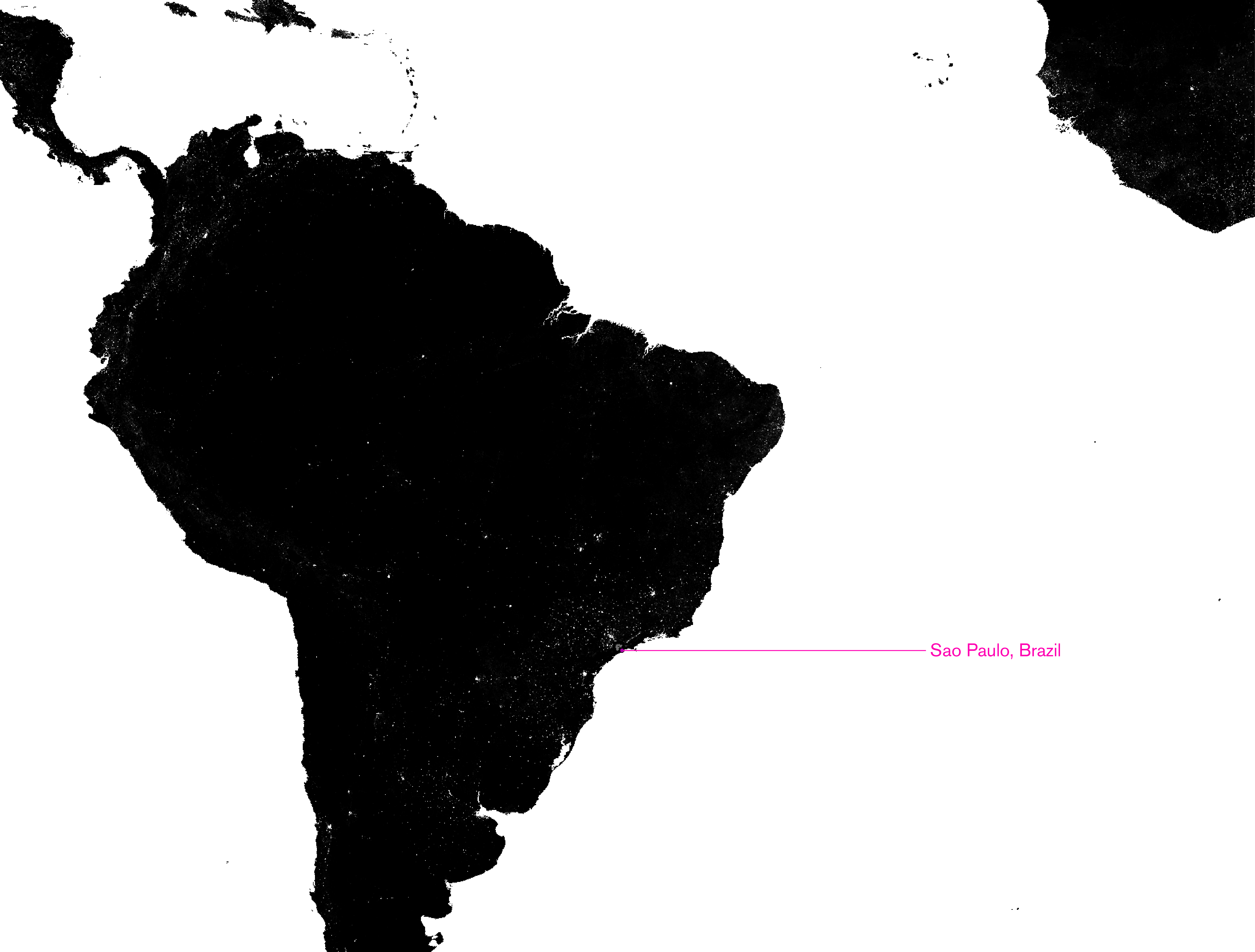
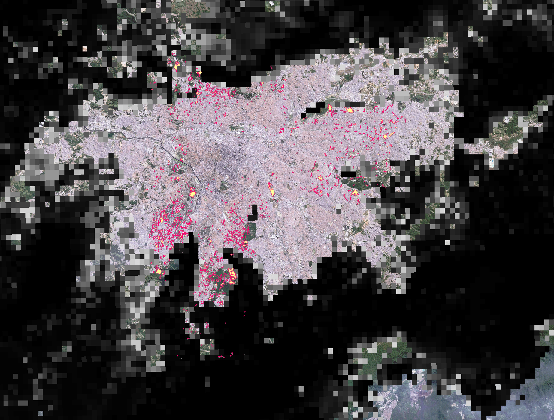
Sao Paulo, Brazil
Sao Paulo
on the other hand provides us with a more diverse dataset on the very refined mesh
of favelas throughout the city, but in a completely different environment in terms of
topography and landscape. These two rates averaged together provide a more
subjective rate number that better reflects the rate of population growth of slums.

However, besides physical quantities, by looking further into the main differences between formal and informal development, we can identify additional variables that affect the growth of slums. In rational, traditional planning, what is generally followed is a top-down approach, with centralized and direct rules that determine the spatial organization, arrangement and order of the cityscape, whereas with informality, a spatial condition is generated by different socioeconomic, unregulated and disorganized principles. The resulting marginalized microcosms vary greatly from city to city and describing more accurately how some of these parameters, weighted and statistically manipulated, contribute to their evolution and development, are vital to understanding how slums form and evolve in different regions. A foreseeable stepping stone of this investigation is the incorporation of a slope/steepness constant that will be user defined, therefore allowing the modification of the outcome depending on user’s requirements. While the algorithmic analysis of the slum will not formalize its development, predicting potential growth in a given environment can assist in the creation of formal development and governing principles that are more informed and can negotiate the parallel existence of a potential secondary fabric more effectively. Additionally, an algorithmic model of informal urban growth can shed light on trends and policies aimed at eliminating slums as part of the belief that they constitute a social problem. Redevelopment has been “all the rage” in recent years, falling under a neoliberal agenda or more particular, hyper-capitalistic trends that utilize such spaces to maximize profit. However, the direct clash between such ambitious visions and the vast bureaucracy that tethers the regions under consideration, or political agendas working against them make it difficult to implement and strategize redevelopment schemes.
Methodology:
The parameters that were selected as inputs for this model were deemed the most
influential in shaping the slums to their current state and carry significant weight in
the accuracy of an algorithmic model of this nature. The bulk of the census data for
Sao Paulo and Dharavi were generated using set polygons on census maps in
ArcMap from 2000 and projections of the following decade. The source of error that
might have arose in the estimates was fitted and minimized before published, and is
therefore not considered in the following study (UN World Bank 2000). This data will
be minimized and take the form of two constants, namely a population growth rate and density growth rate. The following equation describes how population growth is
obtained for each year:
$$N_{p} = (\gamma + 1)N_{p-1} (Eq. 1)$$
for each time step,
$$N_{initial-final} = \frac{N_{2}-N_{1}}{N_{1}}100\% (Eq. 2)$$
The Dharavi District slums and Sao Paulo favelas were extracted based on GIS data
that already outlined the main areas and factored in the minuscule adjustments in
size change over that time period. The decade 2000-2010 was chosen among a set
of this and the two decades before it, based on its relative stability in slum size. A
growing area would introduce problems since the data would be extracted over the
original polygon sets, ignoring the expansion of the slum outside it, thus giving us a
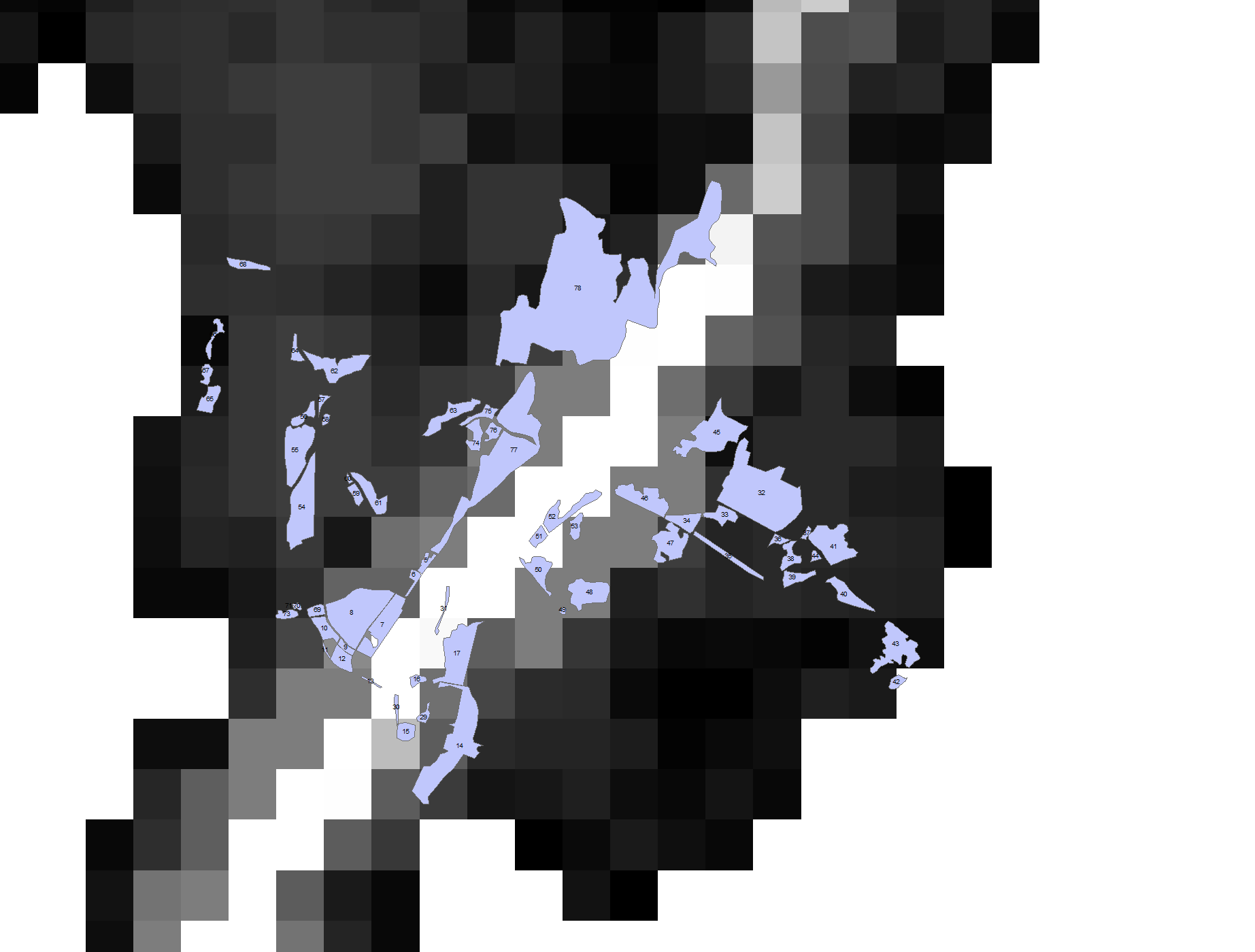
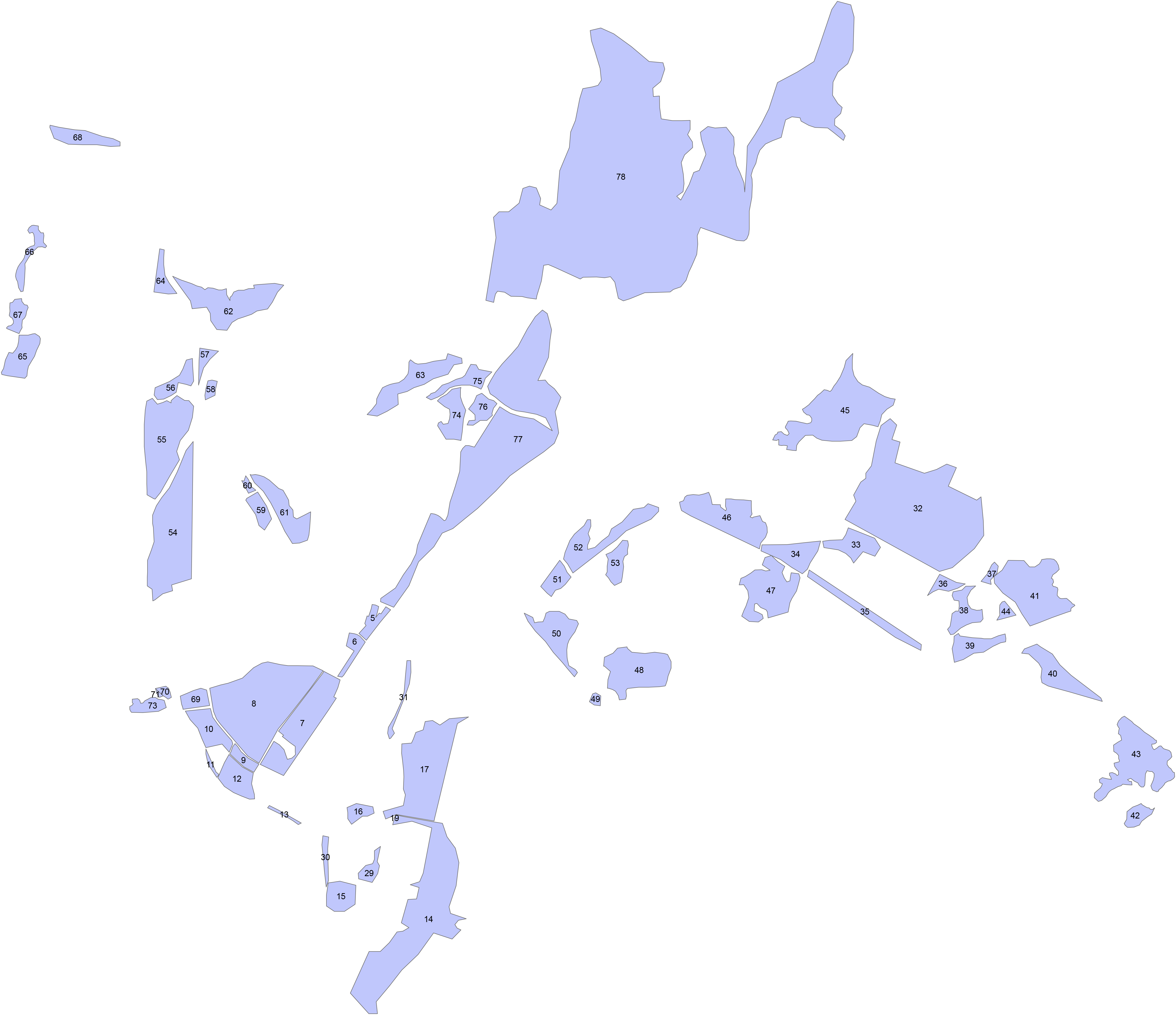
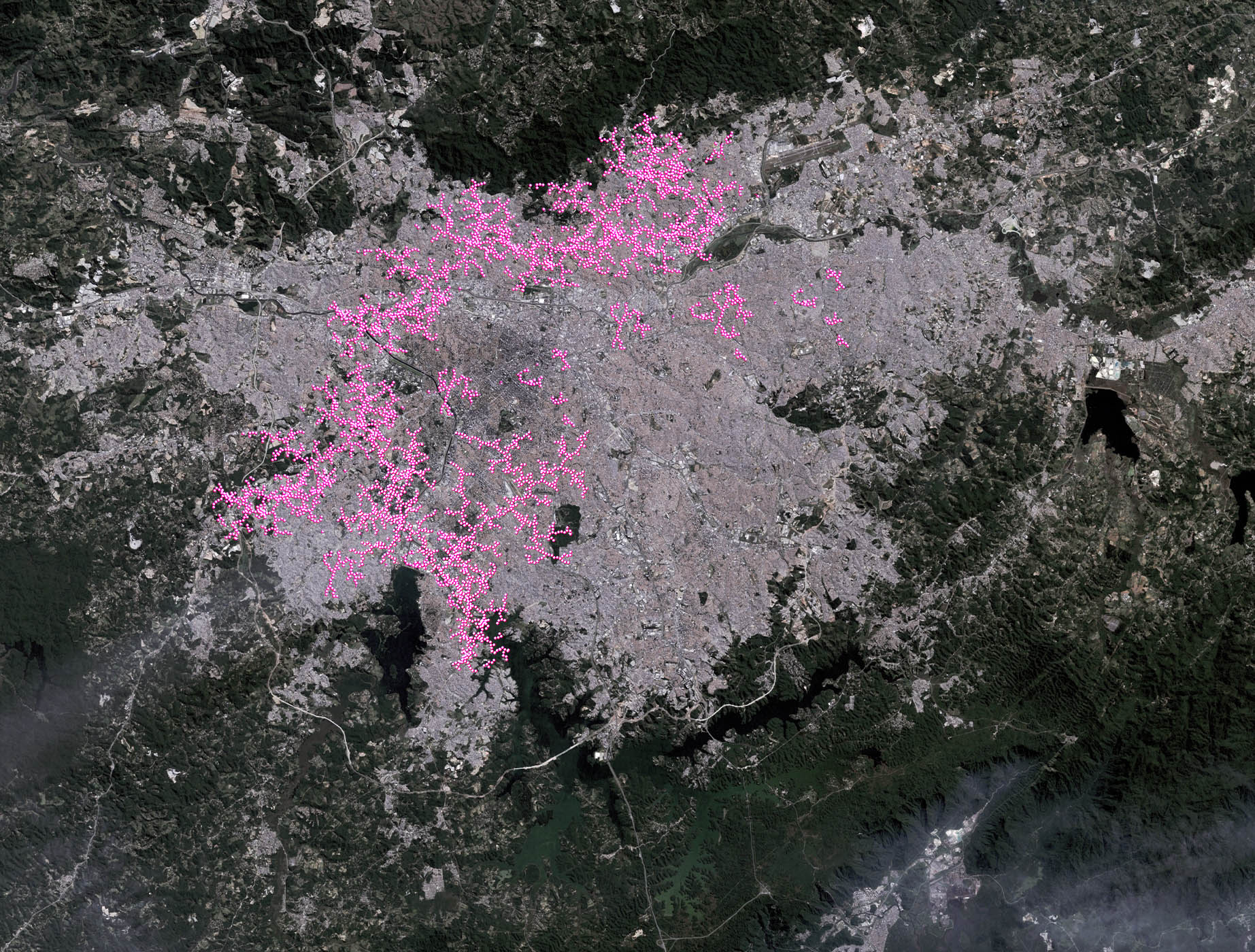
partial answer. Figures 1 and 5 show the polygons that were analyzed in Sao
Paulo and Dharavi respectively:

It is worth noting the directionality of the slums in the picture above; an indication of where the slums started and how they progressed throughout the city or spawned at a later time in different areas can is the density of the polygon sets. The lower left region is a densely packed area that precedes the areas at the top right and upper left sets, as they have existed since the “lost decade of the 1980’s”, when favelas started appearing in the city (UN HABITAT Global Report, 2003). If such evidence is found in a computer model could mean that the latter has an implication that makes it accurate and therefore stands as one of many satisfactory benchmarks for the accuracy of the simulation.
Similarly, for the Dharavi model (Fig.1) we can see natural obstructions within the urban fabric that act as a boundary value when translated in a mathematical model. Fig. 1 shows the collection of polygons that the population data was extracted superimposed on a pixelated morphologically accurate census map that shows Mumbai’s Mithi river in white pixels. Once the boundaries have been introduced in a mathematical model, tracking the proximity of the value to the boundary and whether the model can handle the limit values at the critical points also provides a benchmark that tests the overall accuracy of the model.
Methodology: GIS Data
The nine time steps obtained using equation 2 were averaged together for each city and yielded the following population growth rates (Appendix 1 contains the raw data for the Dharavi district as a reference of how the constants were obtained):
| Population | Increase | Rate (%) | Area | Density | Rate (%) | |
|---|---|---|---|---|---|---|
| 2000 | 434277 | NA | NA | 1034 | 419.9970986 | NA |
| 2001 | 446333 | 12056 | 2.776108336 | 1034 | 431.6566731 | 2.776108336 |
| 2002 | 446806 | 473 | 0.105974687 | 1034 | 432.1141199 | 0.135974687 |
| 2003 | 453527 | 6721 | 1.504232262 | 1034 | 438.6141199 | 1.904232262 |
| 2004 | 483801 | 30274 | 6.675236535 | 1034 | 467.8926499 | 6.635236535 |
| 2005 | 518799 | 34998 | 7.233966031 | 1034 | 501.7398453 | 7.233966031 |
| 2006 | 536203 | 17404 | 3.354671077 | 1034 | 518.5715667 | 3.154671077 |
| 2007 | 563028 | 26825 | 5.002769474 | 1034 | 544.5145068 | 5.002769474 |
| 2008 | 572003 | 8975 | 1.594059265 | 1034 | 553.1943907 | 2.594059265 |
| 2009 | 580100 | 8097 | 1.415552016 | 1034 | 561.0251451 | 1.815552016 |
| 2010 | 608465 | 28365 | 4.889674194 | 1034 | 588.4574468 | 5.089674194 |
| Average | N/A | 17419 | 3.45524 | N/A | 496.1616 | 3.49294 |
| Population | Increase | Rate (%) | Area | Density | Rate (%) | |
|---|---|---|---|---|---|---|
| 2000 | 1226773 | NA | NA | 102 | 12027.18627 | NA |
| 2001 | 1281552 | 54786 | 4.275342 | 102 | 12564.23529 | 4.465292275 |
| 2002 | 1352475 | 70921 | 5.2437455 | 102 | 13259.55882 | 5.534149219 |
| 2003 | 1382091 | 29618 | 2.1435679 | 102 | 13549.91176 | 2.189763212 |
| 2004 | 1426670 | 44576 | 3.1245789 | 102 | 13986.96078 | 3.225475023 |
| 2005 | 1489747 | 63029 | 4.2315436 | 102 | 14605.36275 | 4.421274717 |
| 2006 | 1609659 | 119912 | 7.4528435 | 102 | 15780.97059 | 8.04915197 |
| 2007 | 1719880 | 110279 | 6.4124335 | 102 | 16861.56863 | 6.847475148 |
| 2008 | 1795472 | 75589 | 4.2143532 | 102 | 17602.66667 | 4.395190362 |
| 2009 | 1889970 | 94498 | 5.0034222 | 102 | 18529.11765 | 5.263128581 |
| 2010 | 1980456 | 90485 | 4.5689789 | 102 | 19416.23529 | 4.787695043 |
| Average | N/A | 17419 | 4.66708 | N/A | 15289.43405 | 4.917859555 |
$$N_{p} = 4.06116 (Eq. 3)$$
Similarly, the density increase rate parameter is the statistical average of the two values:
$$D_{p} = 4.2054 (Eq. 4)$$
Methodology: Topographic Condition Constant
A defining parameter that influences formal construction is the morphology of the
surrounding landscape. With spontaneously spawning structures such as slums, the
amount of construction is similarly defined by the steepness of the landscape in a
linear way i.e. increased slope increases the difficulty of construction. This can be
deduced from materials analyses in smaller scales and then generalized for larger
scale structures, by nature of the quantized matter that they are composed of
(Engineering Materials I 68, 2012). Gravel size data used in the Oklahoma Forestry
Services analysis on construction techniques and cost estimates for large rocked
fords for various stream and road conditions is valuable in creating a correlation between the type of slope and the amount of gravel used in each terrain. Figures
6(a) 6(b) and 6(c) show three different types of terrains and the respective gravel
size used in each step:


$$X_{i, 0,1} = \frac{x_{i}-x_{min}}{x_{max}-x_{min}} (Eq. 4)$$
We obtain the data points \(X_{1} = 0\) for a low slope, \(X_{2} = 0.64\) for a moderate slope and \(X_{3} = 1\) for a steep slope. The increments in between provide a wide range in the normalized scale that covers more specific scenarios per the user requirements. All of the following constant definitions can now be used in a form-generating algorithm that implements them within the statistical fitting. Before implementing the algorithm fully however, its scalability has to be tested in order to verify the implications of the proof of concept. An initial model that creates an initial geometry will therefore be implemented.
Experiments:
The initial run is shown in Figures 7. The directionality of the geometry despite the lack of boundaries in the code is promising, emphasizing on the spatial and temporal resolution that is sufficient enough to extrapolate a valid result. Additionally, the density of the spheres hints at the spatial characteristics of the slums under investigation, particularly the density of the structures at hand. The positions of the structures that appear first at the beginning of the iteration will be then reused by additional spheres that will later be spawned, simulating a natural increased density in “older” structures in the model. While this iteration of the software lacks the level of accuracy that a more refined version will acquire, it provides proof of principle that deems the scalability of the algorithm worthy of analysis.
Team:
Final project, individual.
Tools & methods:
Rhinoceros, Grasshopper, ArcGIS, Rhinoscriptsyntax, Python, Photoshop, Illustrator, InDesign.