Mean-Variance efficient portfolio construction:
This project explores the construction and analysis of mean-variance efficient portfolios using monthly return data for 10 value-weighted industry portfolios drawn from the Fama-French data library, spanning a 90-year historical period. The analysis is implemented in MATLAB's numerical computing environment and covers the full lifecycle of mean-variance portfolio theory: from the Lagrangian derivation of the minimum variance optimization problem, through the closed-form solution for the efficient frontier, to the practical computation of the Minimum Variance Portfolio (MVP) and the Tangency Portfolio — the portfolio on the efficient frontier with the highest Sharpe ratio.
A central theme of the project is estimation risk: the sensitivity of optimal portfolio weights to errors in the estimated expected return vector and covariance matrix. Because these inputs must be estimated from historical data, they are subject to substantial sampling variability — and mean-variance optimization is notorious for amplifying estimation errors, particularly in the tangency portfolio weights. The project investigates this problem through two complementary simulation methodologies: a parametric Monte Carlo approach that draws from a multivariate normal distribution calibrated to historical estimates, and a non-parametric bootstrap that resamples directly from the empirical return distribution without imposing any distributional assumption. The results, following the methodology of Jorion (1992), illustrate quantitatively why the minimum variance portfolio is far more robust to estimation error than the tangency portfolio, and why ex-post mean-variance optimal portfolios systematically overstate the achievable gains from diversification.
Definitions:
Mean-Variance Mathematics:
We define the following elements that will help with the derivation of the mean-variance mathematics we will be using in our computations:
Portfolio weight vector:
$$w_{p}=\begin{bmatrix}w_{1,p}\\w_{2,p}\\.\\.\\.\\w_{n,p}\end{bmatrix}$$
Expected Return Vector:
$$R=\begin{bmatrix}\bar{r_{1}}\\\bar{r_{2}}\\.\\.\\.\\\bar{r_{n}}\end{bmatrix}$$
Covariance Matrix:
$$V=\begin{bmatrix}\sigma_{11}&\sigma_{12}&.&.&.&\sigma_{1N}\\\sigma_{21}&\sigma_{22}&.&.&.&\sigma_{2N}\\.&.&.& & &. \\.&. & &.& &. \\.&. & & &.&. \\\sigma_{N1}&\sigma_{N2}&.&.&.&\sigma_{NN}\end{bmatrix}$$
Unit vector:
$$\textbf{I}=\begin{bmatrix}1\\1\\.\\.\\.\\1\end{bmatrix}$$
Objective function:
The goal is to minimize \(w'Vw\) such that \(w'R=r_{p}\). (Note that \(w'R\) is the weighted mean of the expected return vector).
Deriving the Minimum Variance Portfolio:
Using the Lagrangian method, we solve
$$\mathcal{L}=w'Vw-\lambda_{1}(w'R-r_{p}-\lambda_{2}(w'\textbf{I}-1))$$
Taking the partial derivative with respect to \(w\) yields
$$\frac{\partial \mathcal{L}}{\partial w}=2Vw-\lambda_{1}R-\lambda_{2}\textbf{I}$$ $$\leftrightarrow Vw=\frac{1}{2}\lambda_{1}R+\lambda_{2}\textbf{I}$$ $$\leftrightarrow w^{*}=\frac{1}{2}V^{-1}\lambda_{1}R+\lambda_{2}\textbf{I}$$ $$\leftrightarrow w^{*} = \frac{1}{2}V^{-1}(R\textbf{I})\begin{bmatrix}\lambda_{1}\\\lambda_{2}\end{bmatrix}$$ $$\leftrightarrow (R\textbf{I})'w=\frac{1}{2}\underbrace{(R\textbf{I})'V^{-1}(R\textbf{I})}_{A}\begin{bmatrix}\lambda_{1}\\\lambda_{2}\end{bmatrix}$$ $$A^{-1}(R\textbf{I})'w=\frac{1}{2}\begin{bmatrix}\lambda_{1}\\\lambda_{2}\end{bmatrix}$$ $$w^{*} = V^{-1}(R\textbf{I})A^{-1}\begin{bmatrix}r_{p}\\1\end{bmatrix}$$
The final portfolio weights matrix is therefore
$$\boxed{w^{*} = V^{-1}(R\textbf{I})A^{-1}\begin{bmatrix}r_{p}\\1\end{bmatrix}}$$ We are assuming that V is positive semidefinite i.e. invertible and multiply by V^{-1} in line 3.
A is the fundamental matrix $$A = (R\textbf{I})'V^{-1}(R\textbf{I})$$
$$\leftrightarrow \begin{bmatrix}R'V^{-1}R & \textbf{I}'V^{-1}R\\R'V^{-1}\textbf{I} & \textbf{I}V^{-1}\textbf{I}\end{bmatrix}$$
$$\boxed{A=\begin{bmatrix}a & b\\c & d\end{bmatrix}}$$ The variance of the portfolio is
$$\sigma^{2}_{p}=w'Vw=$$
$$\underbrace{\begin{bmatrix}r_{p} & 1\end{bmatrix}A^{-1}(R\textbf{I})V^{-1}}_{w'}\ V \ \overbrace{V^{-1}(R\textbf{I})A^{-1}\begin{bmatrix}r_{p}\\ 1\end{bmatrix}}^\text{w}$$
$$\leftrightarrow \begin{bmatrix}r_{p}&1\end{bmatrix}A^{-1}AA^{-1}\begin{bmatrix}r_{p}\\1\end{bmatrix}$$
$$\leftrightarrow \begin{bmatrix}r_{p}&1\end{bmatrix}A^{-1}\begin{bmatrix}r_{p}\\1\end{bmatrix}$$
$$\sigma^{*2}_{p}=\begin{bmatrix}r_{p} & 1\end{bmatrix}\underbrace{\frac{\begin{bmatrix}c & -b\\-b & a\end{bmatrix}}{ac-b^2}}_{A^{-1}}\begin{bmatrix}r_{p}\\ 1\end{bmatrix}$$
$$\leftrightarrow \frac{\begin{bmatrix}cr_{p}-b & -br_{p}+a\end{bmatrix}}{ac-b^{2}}\begin{bmatrix}r_{p}\\1\end{bmatrix}$$
$$\leftrightarrow \frac{cr_{p}-br_{p}-br_{p}+a}{ac-b^{2}}$$
$$\sigma^{*2}_{p}=\frac{a-2br_{p}+cr_{p}}{ac-b^{2}}$$
The minimum variance portfolio is therefore $$\boxed{\sigma^{*2}_{p}=\frac{a-2br_{p}+cr_{p}}{ac-b^{2}}}$$
(Note that \(\sigma^{*2}_{p}\) is a parabolic function).
We can further simplify the expression as follows:
$$\frac{\partial \sigma^{2}_{p}}{\partial r_{p}}=-2b+2cr_{p}=0$$
$$ \leftrightarrow r_{p}=\frac{b}{c}$$
$$r_{MVP}=\frac{b}{c}=\frac{\textbf{I}'V^{-1}R}{\textbf{I}'V^{-1}\textbf{I}}=w_{MVP}'R$$
$$\leftrightarrow (\frac{\textbf{I}'V^{-1}}{\textbf{I}'V^{-1}\textbf{I}})R=w_{MVP}'R$$
$$\sigma^{2}_{MVP}=w_{MVP}'Vw_{MVP}=(\frac{\textbf{I}'V^{-1}}{\textbf{I}'V^{-1}\textbf{I}})'V\frac{\textbf{I}'V^{-1}}{\textbf{I}'V^{-1}\textbf{I}}$$
$$\sigma^{2}_{MVP}=\frac{\textbf{I}}{\textbf{I}'V^{-1}\textbf{I}}=\frac{1}{c}$$
$$\boxed{\sigma^{2}_{MVP}=\frac{1}{c}}$$
Finally the Minimum Variance Portfolio is defined as $$\boxed{\sigma^{*2}_{p}=\frac{a-2br_{p}+cr_{p}}{ac-b^{2}}=\frac{1}{c}}$$
We can also prove that the covariances between stock returns and returns of the Minimum Variance Portfolio is the same across all stocks: $$Cov(R_{p},R_{MVP})=Cov(R_{q},R_{MVP})=\sigma^{2}_{MVP}\forall p,q$$
Proof: $$\sigma^{2}_{MVP}=w_{p}'Vw_{MVP}$$ $$\leftrightarrow w_{p}'V(\frac{\textbf{I}'V^{-1}}{\textbf{I}'V^{-1}\textbf{I}})=\frac{w^{'}_{p}\textbf{I}}{\textbf{I}'V^{-1}\textbf{I}}$$ $$\leftrightarrow \frac{1}{\textbf{I}'V^{-1}\textbf{I}}=\frac{1}{c}$$
Summary:
MVP:
- $$\leftrightarrow w=\frac{V^{-1}\textbf{I}}{\textbf{I}V^{-1}\textbf{I}}=w_{MVP}$$ $$\boxed{\frac{1}{\sigma_{i,MVP}}=\frac{1}{\sigma_{k,MVP}}\forall i,k}$$
Tangency Portfolio (hereinafter referred to as TP; The TP is defined as the portfolio on the efficient frontier with the lowest Sharpe Ratio):
- $$w'V=(R-r_{f}\textbf{I})$$ $$\boxed{w=\frac{V^{-1}(R-r_{f}\textbf{I})}{(\textbf{I}V^{-1}(R-r_{f}\textbf{I})}=w_{TANG}}$$
- $$\boxed{\frac{\textbf{E}[r_{i}]-r_{f}}{\sigma_{i,TANG}}=\frac{\textbf{E}[r_{k}]-r_{f}}{\sigma_{k,TANG}}}$$where \(r_{f}\) is the risk-free rate. In essence, the above equation tells us that the marginal Sharpe ratios are equal across all stocks within the portfolio.
Programming:
We will now be using the variance mathematics derived above to compute the efficient frontier and other useful metrics:
      clc;
      clear all;
      close all;
      dates = table2array(readtable('10_data.xls','Range','A22:A1090','ReadVariableNames',false));
      industries = table2array(readtable('Problem_Set2.xls','Range','B22:K1090','ReadVariableNames',false));
      Rf = table2array(readtable('Problem_Set2.xls','Range','L22:L1090','ReadVariableNames',false));
      industry_names = {'NoDur'; 'Durbl'; 'Manuf'; 'Enrgy'; 'HiTec'; 'Telcm'; 'Shops'; 'Hlth '; 'Utils'; 'Other'};
      T = size(industries,1);                   % Number of Rows
      N = size(industries,2);                   % Number of Columns (Number of industries)
      R = mean(industries)';                    % Expected Return Vector
      Var = var(industries);                    % Variance Matrix
      Std = sqrt(Var);                          % Standard Deviation Vector
      Unit = ones(10,1);                        % Ones column
      V = cov(industries);                      % Covariance Matrix
      A = [R Unit]'*inv(V)*[R Unit];            % Fundamental Matrix
      Rf = mean(Rf); % Risk-free rate average
      w_mvp = (inv(V)*Unit)/(Unit'*inv(V)*Unit);
      w_tang = (inv(V)*(R-Rf*Unit))/(Unit'*inv(V)*(R-Rf*Unit));
      col_names = {'MVP'; 'Tangency'};
      weight_table = table(w_mvp,w_tang);
      weight_table.Properties.RowNames = industry_names;
      weight_table.Properties.VariableNames = col_names;
      disp('Question 1: Weights of the Minimum Variance & Tangency Portfolios')
      weight_table

                  MVP       Tangency
               _________    _________
      NoDur       0.7746      0.82129
      Durbl    -0.060079     0.095072
      Manuf     -0.12834     -0.19566
      Enrgy      0.22043      0.31653
      HiTec     -0.10569      0.01979
      Telcm      0.55252      0.33927
      Shops    -0.060366    -0.041804
      Hlth      0.070014      0.32376
      Utils     0.075914    -0.034497
      Other     -0.33899     -0.64375
Comments:
The weights of the industries in the MVP and the TP are substantially different, with the TP weights having more extreme values than the weights in the MVP.
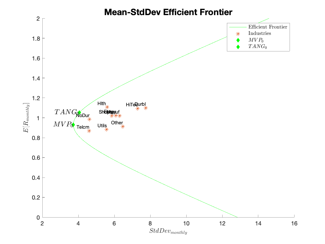
We now compute the means and standard deviations of the MVP and TP and plot the efficient frontier of the 10 industries on a mean-standard deviation diagram:
          rp_mvp = w_mvp'*R;
          rp_tang = w_tang'*R;
          var_mvp = w_mvp'*V*w_mvp;
          var_tang = w_tang'*V*w_tang;
          sd_mvp = sqrt(var_mvp);
          sd_tang = sqrt(var_tang);
          stats_mvp = [sd_mvp rp_mvp];
          stats_tang = [sd_tang rp_tang];
          stats = [stats_mvp;stats_tang];
          rp_frontier = linspace(0,2,5000);
          v_frontier = [];
          for i = 1:5000
              v_frontier(i) = [rp_frontier(i) 1]*inv(A)*[rp_frontier(i) 1]';
          end
          std_frontier = sqrt(v_frontier);
          q1a = figure;
          figure(q1a);
          hold on
          plot(std_frontier,rp_frontier,'green');
          scatter(Std,R','*');
          text(Std+0.01',R'+0.01,industry_names,'FontSize',7,'HorizontalAlignment','right','VerticalAlignment','bottom');
          scatter(stats(1,1),stats(1,2),'d','filled','green');
          text(stats(1,1),stats(1,2),'$MVP_\mathrm{0}$','FontSize',12,'HorizontalAlignment','right','Interpreter', 'latex');
          scatter(stats(2,1),stats(2,2),'d','filled','green');
          text(stats(2,1),stats(2,2),'$TANG_\mathrm{0}$','FontSize',12,'HorizontalAlignment','right','Interpreter', 'latex');
          xlabel('$StdDev_{monthly}$', 'Interpreter', 'latex');
          ylabel('$E[R_{monthly}]$', 'Interpreter' , 'latex');
          legend('Efficient Frontier','Industries','$MVP_\mathrm{0}$','$TANG_\mathrm{0}$','Interpreter', 'latex');
          title('Mean-StdDev Efficient Frontier','FontSize',15);
          hold off
Mean-Std Efficient Frontier:
          Std_Error = Std/sqrt(N);
          R_error = R+Std_Error';
          w_tang_error = (inv(V)*(R_error-Rf*Unit))/(Unit'*inv(V)*(R_error-Rf*Unit));
          rp_tang_error = w_tang_error'*R_error;
          var_tang_error = w_tang_error'*V*w_tang_error;
          sd_tang_error = sqrt(var_tang_error);
          stats_tang_error = [sd_tang_error rp_tang_error];
          stats_error_1b = [stats_mvp;stats_tang_error];
          A_error = [R_error Unit]'*inv(V)*[R_error Unit];                    % Modified Fundamental Matrix
          rp_frontier_error = linspace(0,4,5000);
          v_frontier_error = [];

          for i = 1:5000
              v_frontier_error(i) = [rp_frontier_error(i) 1] * inv(A_error)*[rp_frontier_error(i) 1]';
          end

          std_frontier_error = sqrt(v_frontier_error);

          q1b = figure;
          figure(q1b);
          hold on
          plot(std_frontier,rp_frontier,'green');
          plot(std_frontier_error,rp_frontier_error,'red')
          scatter(Std,R_error','*')
          text(Std+0.01',R_error'+0.01,industry_names,'FontSize',8,'HorizontalAlignment','right','VerticalAlignment','bottom','Interpreter', 'latex');
          scatter(stats(2,1),stats(2,2),'d','filled','green');
          text(stats(2,1),stats(2,2),'$TANG_\mathrm{0}$','FontSize',12,'HorizontalAlignment','right','Interpreter', 'latex');
          scatter(stats_error_1b(2,1),stats_error_1b(2,2),'d','filled','green');
          text(stats_error_1b(2,1),stats_error_1b(2,2),'$TANG_\mathrm{+1\sigma_\mathrm{\bar{x}}}$','FontSize',12,'HorizontalAlignment','right','Interpreter', 'latex');
          xlabel('$StdDev_{monthly}$', 'Interpreter', 'latex');
          ylabel('$E[R_{monthly}]$', 'Interpreter' , 'latex');
          legend('Original Efficient Frontier','Efficient Frontier w/ $\mathrm{+1\sigma_\mathrm{\bar{x}}}$','Industries','$TANG_\mathrm{0}$','$TANG_\mathrm{+1\sigma_\mathrm{\bar{x}}}$','Interpreter','latex');
          title('Mean-StdDev Efficient Frontier $\mathrm{+1\sigma_\mathrm{\bar{x}}}$','FontSize',15,'Interpreter', 'latex');
          hold off

                  Historical              Means+1stderror
                  MVP         Tangency    MVP         Tangency
                  _____       _____       _____       _____
          NoDur    0.77        0.82        0.77        0.71
          Durbl   -0.06        0.10       -0.06        0.12
          Manuf   -0.13       -0.20       -0.13       -0.24
          Enrgy    0.22        0.32        0.22        0.32
          HiTec   -0.11        0.02       -0.11        0.04
          Telcm    0.55        0.34        0.55        0.33
          Shops   -0.06       -0.04       -0.06       -0.02
          Hlth     0.07        0.32        0.07        0.31
          Utils    0.08       -0.03        0.08       -0.00
          Other   -0.34       -0.64       -0.34       -0.56
Mean-Std Efficient Frontier +1 Standard Error:
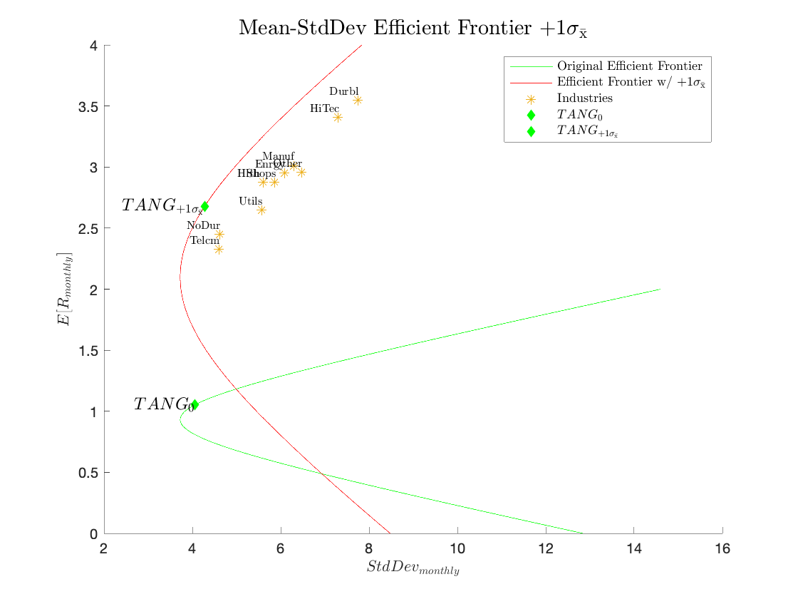
Comments:
The standard errors suggests that none of the means are statistically significant from each other (within 2 standard errors). This lack of statistical significance to the difference in estimated means is important because the tangency portfolio will heavily weight those industries which appear to have high means and often suggest shorting those industries which appear to have low means. If in fact the apparent difference in means is just noise, the tangency portfolio will thus be very affected by it. The table above lists the Historical means for the MVP and TP as well as the corresponding results for the means+1 standard error.
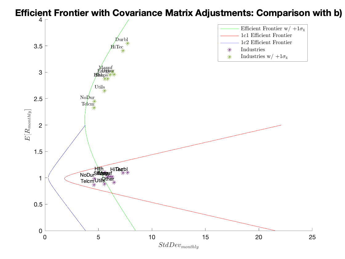
Since we are relying heavily on the covariance matrix that we computed, it is prudent to also test its reliability and determine whether our computation is more sensitive to the variance or covariance terms.
          %Covariance Matrix = diag(Var_Matrix)%
          V_Variances = [];                                                     % Covariance Matrix (Diagonal Matrix of Variances)
          for i = 1:10
              V_Variances(i,i) = V(i,i);
          end

          A_diag = [R Unit]'*inv(V_Variances)*[R Unit];                         % Fundamental Matrix 1) c. 1-
          w_mvp_diag = (inv(V_Variances)*Unit)/(Unit'*inv(V_Variances)*Unit);
          w_tang_diag = (inv(V_Variances)*(R-Rf*Unit))/(Unit'*inv(V_Variances)*(R-Rf*Unit));

          rp_mvp_diag = w_mvp_diag'*R;
          rp_tang_diag = w_tang_diag'*R;
          var_mvp_diag = w_mvp_diag'*V_Variances*w_mvp_diag;
          var_tang_diag = w_tang_diag'*V_Variances*w_tang_diag;
          sd_mvp_diag = sqrt(var_mvp_diag);
          sd_tang_diag = sqrt(var_tang_diag);
          stats_mvp_diag = [sd_mvp_diag rp_mvp_diag];
          stats_tang_diag = [sd_tang_diag rp_tang_diag];
          stats_diag = [stats_mvp_diag;stats_tang_diag];
          rp_frontier_diag = linspace(0,2,5000);
          v_frontier_diag = [];

          for i = 1:5000
              v_frontier_diag(i) = [rp_frontier_diag(i) 1]*inv(A_diag)*[rp_frontier_diag(i) 1]';
          end

          std_frontier_diag = sqrt(v_frontier_diag);

          %Covariance Matrix = eye(10,10)%
          V_eye = eye(10,10);                                                   % Covariance Matrix (Identity matrix)
          A_eye = [R Unit]'*inv(V_eye)*[R Unit];                                % Fundamental Matrix 1) c. 2-
          w_mvp_eye = (inv(V_eye)*Unit)/(Unit'*inv(V_eye)*Unit);
          w_tang_eye = (inv(V_eye)*(R-Rf*Unit))/(Unit'*inv(V_eye)*(R-Rf*Unit));
          rp_mvp_eye = w_mvp_eye'*R;
          rp_tang_eye = w_tang_eye'*R;
          var_mvp_eye = w_mvp_eye'*V_eye*w_mvp_eye;
          var_tang_eye = w_tang_eye'*V_eye*w_tang_eye;
          sd_mvp_eye = sqrt(var_mvp_eye);
          sd_tang_eye = sqrt(var_tang_eye);
          stats_mvp_eye = [sd_mvp_eye rp_mvp_eye];
          stats_tang_eye = [sd_tang_eye rp_tang_eye];
          stats_eye = [stats_mvp_eye;stats_tang_eye];
          rp_frontier_eye = linspace(0,2,5000);
          v_frontier_eye = [];

          for i = 1:5000
              v_frontier_eye(i) = [rp_frontier_eye(i) 1]*inv(A_eye)*[rp_frontier_eye(i) 1]';
          end

          std_frontier_eye = sqrt(v_frontier_eye);

          %Covariance Matrix Comparison a)%
          q1c = figure;
          figure(q1c);
          hold on
          plot(std_frontier_error,rp_frontier_error,'green')
          plot(std_frontier_diag,rp_frontier_diag,'red');
          plot(std_frontier_eye,rp_frontier_eye,'blue');
          scatter(Std,R','*');
          text(Std+0.01',R'+0.01,industry_names,'FontSize',7,'HorizontalAlignment','right','VerticalAlignment','bottom');
          scatter(Std,R_error','*')
          text(Std+0.01',R_error'+0.01,industry_names,'FontSize',8,'HorizontalAlignment','right','VerticalAlignment','bottom','Interpreter', 'latex');
          xlabel('$StdDev_{monthly}$', 'Interpreter', 'latex');
          ylabel('$E[R_{monthly}]$', 'Interpreter' , 'latex');
          legend('Efficient Frontier w/ $\mathrm{+1\sigma_\mathrm{\bar{x}}}$','1c1 Efficient Frontier','1c2 Efficient Frontier','Industries','Industries w/ $\mathrm{+1\sigma_\mathrm{\bar{x}}}$','Interpreter', 'latex');
          title('Efficient Frontier with Covariance Matrix Adjustments: Comparison with b)','FontSize',15);
          hold off

          %Covariance Matrix Comparison b)%
          q1c2 = figure;
          figure(q1c2);
          hold on
          plot(std_frontier,rp_frontier,'magenta');
          plot(std_frontier_error,rp_frontier_error,'green')
          plot(std_frontier_diag,rp_frontier_diag,'blue');
          plot(std_frontier_eye,rp_frontier_eye,'red');
          scatter(Std,R','*');
          text(Std+0.01',R'+0.01,industry_names,'FontSize',7,'HorizontalAlignment','right','VerticalAlignment','bottom');
          scatter(Std,R_error','*')
          text(Std+0.01',R_error'+0.01,industry_names,'FontSize',8,'HorizontalAlignment','right','VerticalAlignment','bottom','Interpreter', 'latex');
          xlabel('$StdDev_{monthly}$', 'Interpreter', 'latex');
          ylabel('$E[R_{monthly}]$', 'Interpreter' , 'latex');
          legend('Original Efficient Frontier','Efficient Frontier w/ $\mathrm{+1\sigma_\mathrm{\bar{x}}}$','1c1 Efficient Frontier','1c2 Efficient Frontier','Industries','Industries w/ $\mathrm{+1\sigma_\mathrm{\bar{x}}}$','Interpreter', 'latex');
          title('Efficient Frontier with Covariance Matrix Adjustments: Comparison with 1) a.','FontSize',15);
          hold off
Efficient Frontier with Covariance Matrix Adjustments: Comparison with the +1StdErr-Adjusted EF:
Efficient Frontier with Covariance Matrix Adjustments: Comparison with Original:
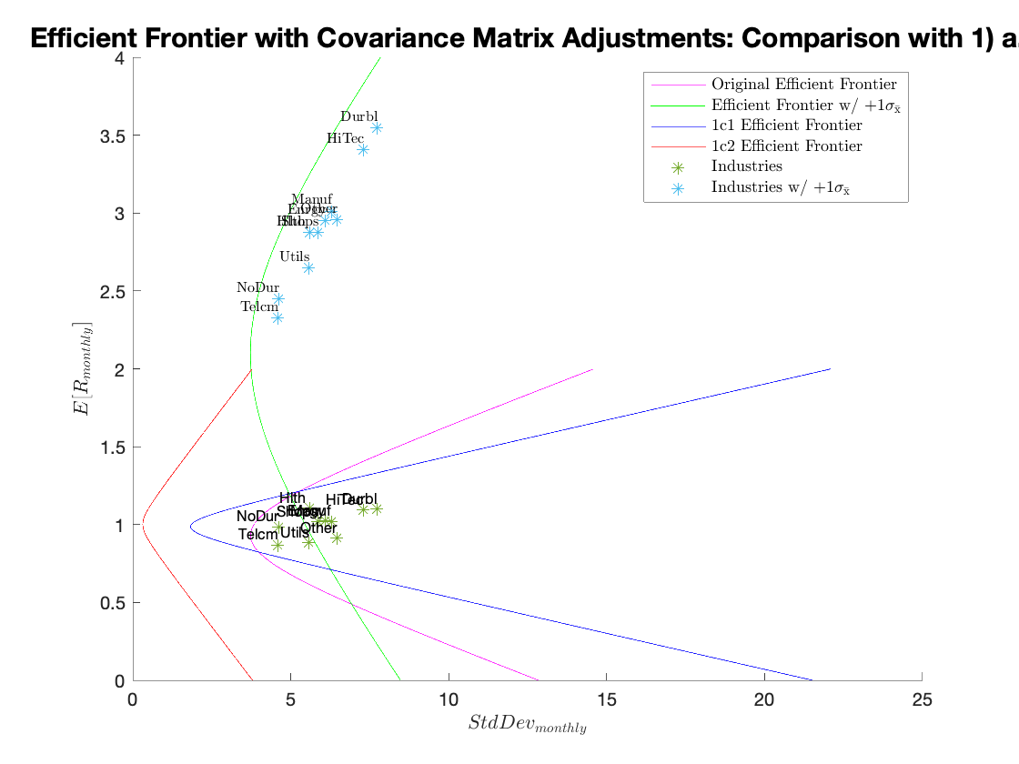
Comments:
The weights change significantly when the covariances are eliminated, and by a marginal amount when the variances are adjusted. The MV and the efficient frontiers are also quite different between the two scenarios. In summary, the covariances are critical in the correct calculation of the efficient frontiers of the MVP and TP, while the variances contribute marginally.
In this section we will be performing simulations similar to Jorion (1992) to further study the effect of measurement error on optimal portfolio allocations.
From the paper:
A major drawback with the classical implementation of mean-variance analysis is that it completely ignores the effect of measurement error on optimal portfolio allocations. A simple simulation approach can provide insight into the distribution of optimal portfolio weights. As an example, an ex post optimal portfolio of U.S. and foreign bonds is compared with two benchmarks- a world bond index and a US. bond index. Taking sampling variability into account, there is no evidence that the optimal portfolio outperformed the world index over the 1978-8 period. The optimal portfolio did, however, perform significantly better than the U.S. index. These results suggest that, over the time period studied, international diversification into foreign bonds has offered some benefits. These benefits are best measured, however, by comparing the performance of a passive world index with that of a US. index. An ex-post mean-variance analysis systematically overstates the possible gains from going international.
Comments:
We only have estimates of the mean returns and covariance matrix of the different industries. We would like to have some idea about the effect of estimation error—what if the truth is different from our estimates? The previous two questions examine changing the estimates and seeing how our portfolios would change. With simulations, we can imagine that we know the truth and then see the magnitude of errors in our estimates and the effects of those estimation errors. This technique gives us the ability to assess deviations from the artificial “truth” that we used to draw the data, using a technique called a parametric Monte Carlo simulation. We use estimates based on actual data as parameters in drawing random variables across different simulation trials. In this case, we are going to imagine that our estimate from the historical data is truth, but then imagine re-running history to see what returns might have been realized given that truth, and thus what we might have estimated, and thus what we might have chosen as MVP and Tangency portfolios.
The real question we have is how much do the weights change, but it is difficult to summarize 10 weights simultaneously. Therefore, the question suggests simply plotting the expected return and standard deviation of the portfolios using the assigned weights.
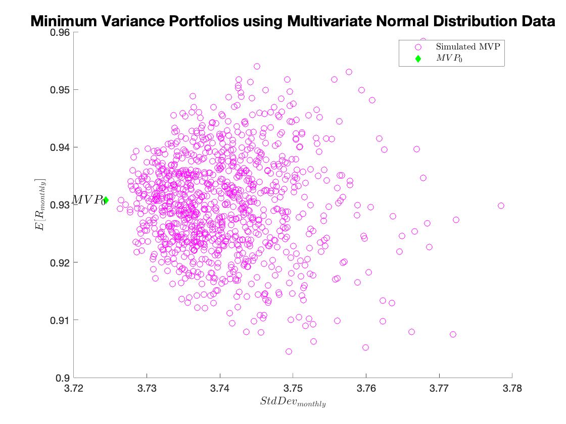
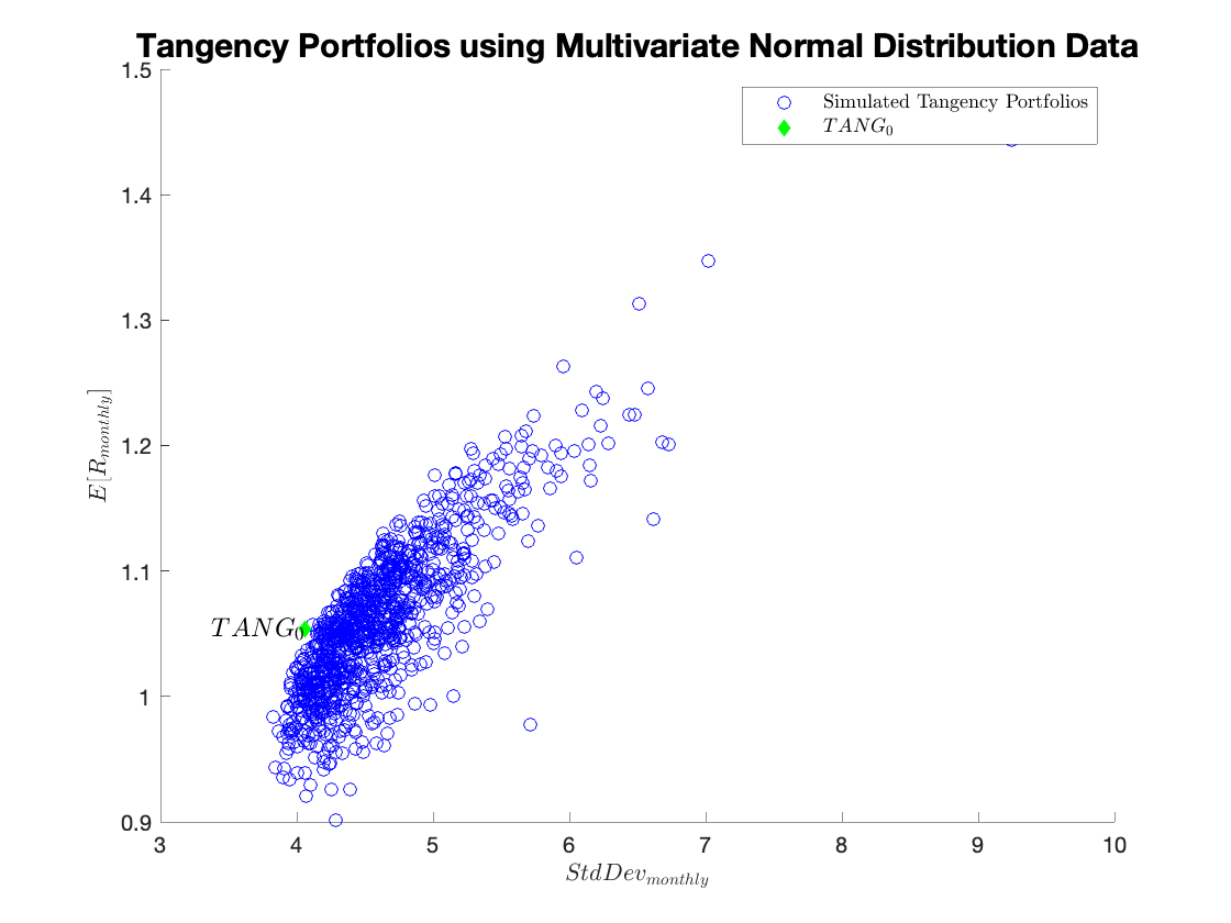
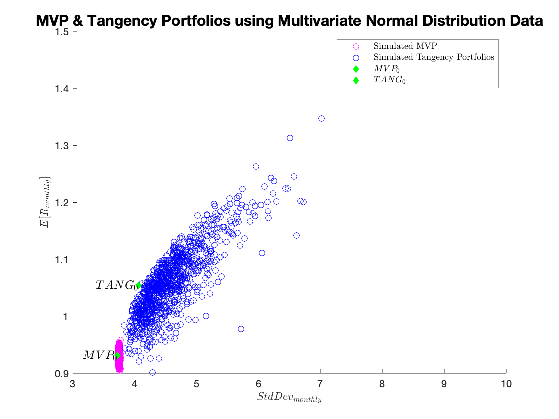
We could plot the expected return and standard deviation using the simulation weights and the simulation estimates of the expected return and standard deviation. Those results are below. Don’t be fooled by the changing x-axis in the two graphs: the lesson is that while the minimum variance portfolio changes a bit, the tangency portfolio changes very much. But in this simulation, we actually know the true (for the simulation) expected return and covariance of the returns. Therefore, we can apply the simulation weights to the true returns and thus get a very clear picture of how much estimation error would cost us in this simulated world. As intuition would suggest, the simulation weights all result in higher variance for the MVP than the weights constructed with knowledge of the truth. Similarly, no portfolio has a higher Sharpe ratio than the true Tangency Portfolio. Overall, these results tell a similar story to the pictures using simulated estimates: while the minimum variance portfolio is not affected much by estimation error, the tangency portfolio is greatly affected by estimation error.
With the existing mean and covariance matrix from the historical data, we generate simulated data under a multivariate normal distribution:
      %Simulated Data%
      rp_mvp_sim = [];
      rp_tang_sim = [];
      sd_mvp_sim = [];
      sd_tang_sim = [];

      %Simulation Procedure%
      for i = 1:1000
          simulated_data = mvnrnd(R',V,T);
          %Mean returns of the siulated data
          R_sim = mean(simulated_data)';

          %Weights of the simulated MVP and Tangency Portfolios
          w_mvp_sim = (inv(cov(simulated_data))*Unit)/(Unit'*inv(cov(simulated_data))*Unit);
          w_tang_sim = (inv(cov(simulated_data))*(R_sim-Rf*Unit))/(Unit'*inv(cov(simulated_data))*(R_sim-Rf*Unit));

          %Simulated means & standard deviations of the MVP and Tangency Portfolios
          rp_mvp_sim(i) = w_mvp_sim'*R;
          rp_tang_sim(i) = w_tang_sim'*R;
          sd_mvp_sim(i) = sqrt(w_mvp_sim'*V*w_mvp_sim);
          sd_tang_sim(i) = sqrt(w_tang_sim'*V*w_tang_sim);
      end

      %Plots

      %Simulated  MVP%
      q1d_mvp = figure;
      figure(q1d_mvp);
      hold on
      scatter(sd_mvp_sim,rp_mvp_sim,'magenta');
      scatter(stats(1,1),stats(1,2),'d','filled','green');
      text(stats(1,1),stats(1,2),'$MVP_\mathrm{0}$','FontSize',12,'HorizontalAlignment','right','Interpreter', 'latex');
      xlabel('$StdDev_{monthly}$', 'Interpreter', 'latex');
      ylabel('$E[R_{monthly}]$', 'Interpreter' , 'latex');
      legend('Simulated MVP','$MVP_\mathrm{0}$','Interpreter','latex');
      title('Minimum Variance Portfolios using Multivariate Normal Distribution Data','FontSize',15);
      hold off

      %Simulated TANG%
      q1d_tang = figure;
      figure(q1d_tang);
      hold on
      scatter(sd_tang_sim,rp_tang_sim,'blue');
      scatter(stats(2,1),stats(2,2),'d','filled','green');
      text(stats(2,1),stats(2,2),'$TANG_\mathrm{0}$','FontSize',12,'HorizontalAlignment','right','Interpreter', 'latex');
      xlabel('$StdDev_{monthly}$', 'Interpreter', 'latex');
      ylabel('$E[R_{monthly}]$', 'Interpreter' , 'latex');
      legend('Simulated Tangency Portfolios','$TANG_\mathrm{0}$','Interpreter','latex');
      title('Tangency Portfolios using Multivariate Normal Distribution Data','FontSize',15);
      hold off

      %Simulated  All%
      q1d_both = figure;
      figure(q1d_both);
      hold on
      scatter(sd_mvp_sim,rp_mvp_sim,'magenta');
      scatter(sd_tang_sim,rp_tang_sim,'blue');
      scatter(stats(1,1),stats(1,2),'d','filled','green');
      text(stats(1,1),stats(1,2),'$MVP_\mathrm{0}$','FontSize',12,'HorizontalAlignment','right','Interpreter', 'latex');
      scatter(stats(2,1),stats(2,2),'d','filled','green');
      text(stats(2,1),stats(2,2),'$TANG_\mathrm{0}$','FontSize',12,'HorizontalAlignment','right','Interpreter', 'latex');
      xlabel('$StdDev_{monthly}$', 'Interpreter', 'latex');
      ylabel('$E[R_{monthly}]$', 'Interpreter' , 'latex');
      legend('Simulated MVP','Simulated Tangency Portfolios','$MVP_\mathrm{0}$','$TANG_\mathrm{0}$','Interpreter','latex');
      title('MVP & Tangency Portfolios using Multivariate Normal Distribution Data','FontSize',15);
      hold off
Minimum Variance Portfolios using Multivariate Normal Distribution Data:
Efficient Frontier with Covariance Matrix Adjustments: Comparison with Original:
MVP & Tangency Portfolios using Multivariate Normal Distribution Data:
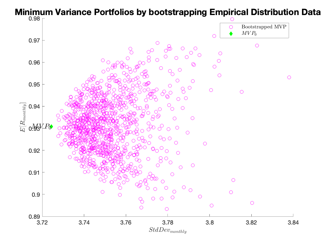
We can continue testing the sensitivity of the MVP and tangency using a non-parametric bootstrap that provides us with more realistic results. We trust that the data constitute a representative sample and we do not force any distribution type on the data (we do not know the specific distribution for the 10-industry data.)
Comments:
In this case, instead of estimating parameters for a normal distribution from the data, we use the empirical distribution directly. This is called a non-parametric bootstrap, and allows us to draw simulated data from the actual data points themselves. (It’s called non-parametric since we do not impose a particular distribution on the data, and thus do not have to estimate parameters for such distributions.) This technique is particularly applicable when we don’t know the true distribution that generated the data, but believe that the sample we collected is a sufficient representation (i.e. representative sample) of the true distribution. We randomly draw 10 returns from the empirical distribution (i.e. from our sample) 947 times. We then use the resulting simulated sample to calculate the tangency and minimum variance portfolios’ weights. This procedure is repeated 1000 times.
%Bootstrapped Data%
rp_mvp_sim = [];
rp_tang_sim = [];
sd_mvp_sim = [];
sd_tang_sim = [];
industries_empirical = [];
%Bootstrapping procedure%
for i = 1:1000
for j = 1:T
r_draw = randi([1 T],1,1);
industries_empirical = [industries_empirical;industries(r_draw,:)];
end
% Mean returns of the bootstrapped data
R_boot = mean(industries_empirical)';
% Weights of the bootstrapped MVP and Tangency Portfolios
w_mvp_boot = (inv(cov(industries_empirical))*Unit)/(Unit'*inv(cov(industries_empirical))*Unit);
w_tang_boot = (inv(cov(industries_empirical))*(R_boot-Rf*Unit))/(Unit'*inv(cov(industries_empirical))*(R_boot-Rf*Unit));
% Bootstrapped means & standard deviations of the MVP and Tangency Portfolios
rp_mvp_boot(i) = w_mvp_boot'*R;
rp_tang_boot(i) = w_tang_boot'*R;
sd_mvp_boot(i) = sqrt(w_mvp_boot'*V*w_mvp_boot);
sd_tang_boot(i) = sqrt(w_tang_boot'*V*w_tang_boot);
industries_empirical = [];
end
% Plots
%Bootstrapped MVP%
q1e_mvp = figure;
figure(q1e_mvp);
hold on
scatter(sd_mvp_boot,rp_mvp_boot,'magenta');
scatter(stats(1,1),stats(1,2),'d','filled','green');
text(stats(1,1),stats(1,2),'$MVP_\mathrm{0}$','FontSize',12,'HorizontalAlignment','right','Interpreter', 'latex');
xlabel('$StdDev_{monthly}$', 'Interpreter', 'latex');
ylabel('$E[R_{monthly}]$', 'Interpreter' , 'latex');
legend('Bootstrapped MVP','$MVP_\mathrm{0}$','Interpreter','latex');
title('Minimum Variance Portfolios by bootstrapping Empirical Distribution Data','FontSize',15);
hold off
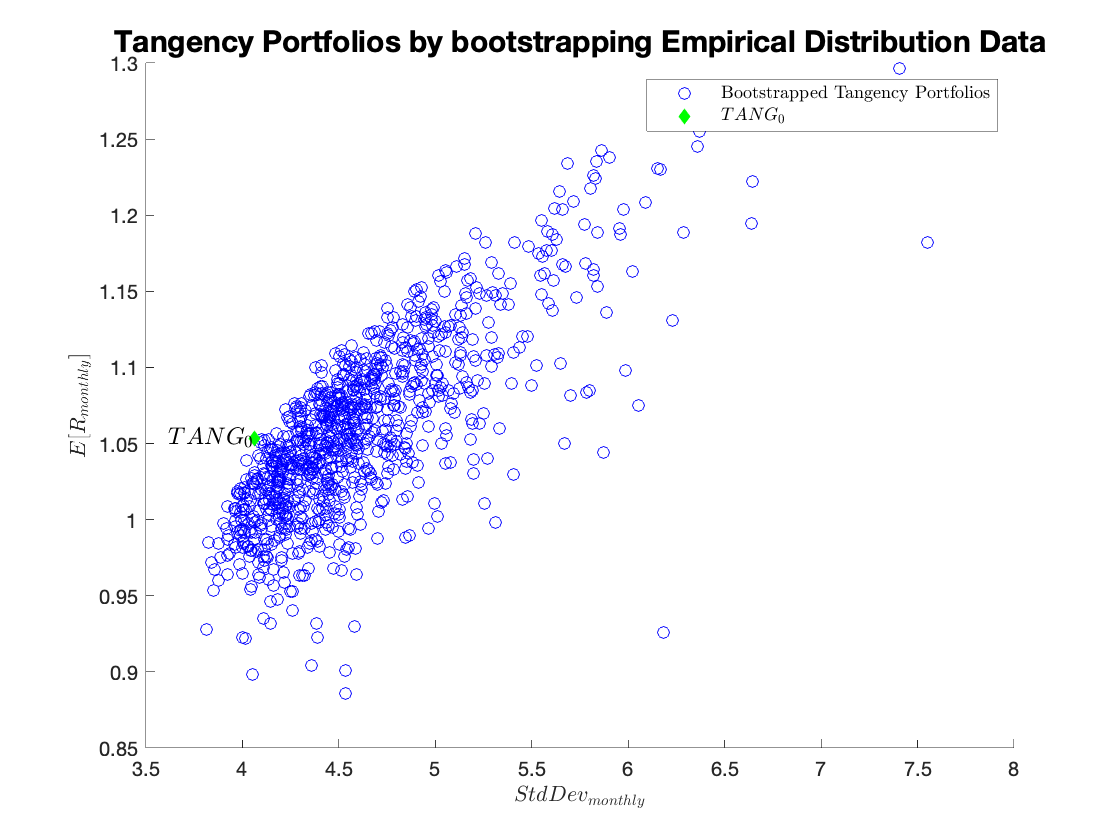
%Bootstrapped TANG%
q1e_tang = figure;
figure(q1e_tang);
hold on
scatter(sd_tang_boot,rp_tang_boot,'blue');
scatter(stats(2,1),stats(2,2),'d','filled','green');
text(stats(2,1),stats(2,2),'$TANG_\mathrm{0}$','FontSize',12,'HorizontalAlignment','right','Interpreter', 'latex');
xlabel('$StdDev_{monthly}$', 'Interpreter', 'latex');
ylabel('$E[R_{monthly}]$', 'Interpreter' , 'latex');
legend('Bootstrapped Tangency Portfolios','$TANG_\mathrm{0}$','Interpreter','latex');
title('Tangency Portfolios by bootstrapping Empirical Distribution Data','FontSize',15);
hold off
%Bootstrapped All%
q1e_both = figure;
figure(q1e_both);
hold on
scatter(sd_mvp_boot,rp_mvp_boot,'magenta');
scatter(sd_tang_boot,rp_tang_boot,'blue');
scatter(stats(1,1),stats(1,2),'d','filled','green');
text(stats(1,1),stats(1,2),'$MVP_\mathrm{0}$','FontSize',12,'HorizontalAlignment','right','Interpreter', 'latex');
scatter(stats(2,1),stats(2,2),'d','filled','green');
text(stats(2,1),stats(2,2),'$TANG_\mathrm{0}$','FontSize',12,'HorizontalAlignment','right','Interpreter', 'latex');
xlabel('$StdDev_{monthly}$', 'Interpreter', 'latex');
ylabel('$E[R_{monthly}]$', 'Interpreter' , 'latex');
legend('Bootstrapped MVP','Bootstrapped Tangency Portfolios','$MVP_\mathrm{0}$','$TANG_\mathrm{0}$','Interpreter','latex');
title('MVP & Tangency Portfolios by bootstrapping Empirical Distribution Data','FontSize',15);
hold off
Minimum Variance Portfolios by bootstrapping Empirical Distribution Data:
Tangency Portfolios by bootstrapping Empirical Distribution Data:
MVP & Tangency Portfolios by bootstrapping Empirical Distribution Data:
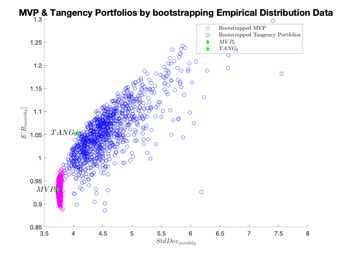
Comments:
Minimum variance portfolio calculations are not very sensitive to the estimation error, but the tangency portfolios are. In fact, the bootstrap simulation seems to be producing larger differences in the inputs, compared to those in the previous simulation. This generates only slightly higher dispersion of the minimum variance portfolio results, but substantially affects tangency portfolios.
Team:
Theodosios Dimitrasopoulos, personal project completed as part of FE 535: Introduction to Financial Risk Management at Stevens Institute of Technology.
Tools & methods:
MATLAB (matrix operations, optimization, Monte Carlo simulation, non-parametric bootstrap), LaTeX (mathematical derivations and report typesetting). The full derivation of mean-variance mathematics follows the Markowitz (1952) framework, with simulation methodology adapted from Jorion (1992) on the effect of measurement error on optimal portfolio allocations.